SILCS-Biologics: Excipient Screening for Biomacromolecular Therapeutics
Background
Biomacromolecular therapeutics, commonly called “biologics,” are typically protein molecules that have been developed to selectively interact with a therapeutic target. Common examples of biologics are therapeutic antibodies. Biologics must be carefully formulated to maximize their stability, so as to ensure both efficacy and safety. Important determinants of stability are protein aggregation and protein denaturation. Toward maximizing stability, biologics can be formulated with excipients, which can help minimize aggregation and denaturation of the biologic in a solution formulation.
SILCS-Biologics applies the patented Site Identification by Ligand Competitive Saturation (SILCS) platform technology to the rational selection of excipients for biologics formulations. The first goal is to minimize protein-protein interactions between multiple molecules of the protein, all in the native state. This reduces the likelihood of aggregation of the protein in its native state. The second goal is to minimize denaturation by stabilizing the native (folded) state of the protein. This is accomplished by screening for excipients that can efficiently bind to the protein native state. Such binding drives the equilibrium toward the native state and away from denatured states. Achieving the second goal also contributes to minimizing aggregation, as denatured states of the protein can be aggregation-prone.
The SILCS-Biologics workflow consists of four steps: 1) SILCS simulation, 2) protein-protein interaction screening, 3) protein-excipient hotspot screening, and 4) analysis and ranking.
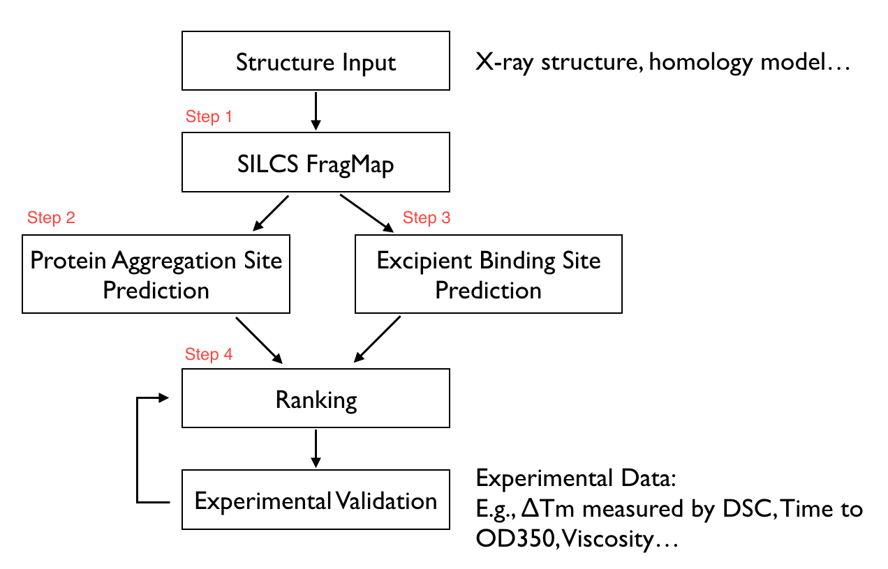
SILCS-Biologics is actualized as a single command-line tool that integrates all four steps. As such, SILCS-Biologics automatically takes care of preparing and running computing jobs that entail SILCS to generate FragMaps, SILCS-PPI to predict protein-protein interactions (PPI) that can drive aggregation, and SILCS-Hotspots to determine excipient binding sites. Please see SILCS: Site Identification by Ligand Competitive Saturation and SILCS-Hotspots: Fragment Binding Sites Including Allosteric Sites for additional details. SILCS-PPI works by aligning FragMaps from one protein with the functional groups on the surface of another protein to predict the likelihood of a PPI between the two proteins [1].
Installation
Please see SilcsBio Software Installation for installation directions for the SilcsBio server software.
Note
SILCS-Biologics is licensed separately from the SILCS platform. Please contact info@silcsbio.com for additional information.
Please contact support@silcsbio.com with installation questions.
Usage
In principle, SILCS-Biologics can be applied to any protein therapeutic. In practice, because SILCS is an all-atom explicit-solvent molecular dynamics methodology, the SILCS simulations underpinning SILCS-Biologics can become computationally prohibitive for large proteins, like full-sequence antibodies or non-antibody protein therapeutics of large size. To enable application of SILCS-Biologics to larger proteins, you may split your full protein into two or three domains. SILCS-Biologics will automatically take care of managing the separate SILCS simulations for each domain and the subsequent SILCS-Hotspots and SILCS-PPI analyses, as well as collating the separate data into a single report for the full-length protein.
In what follows, we discuss three use cases ordered by increasing complexity. The first case involves a protein small enough to be run intact. We use as an example a single Fab fragment (~450 amino acids) from an antibody. The second use case involves a hypothetical fusion protein engineered by combining the sequences of two separate 500 amino acid proteins, with each one forming one domain of the fusion protein. In this second example, the full length protein is first split into its two domains, and each domain is processed as a separate input for computational expediency. The third example is a complete antibody molecule (~1300 amino acids). It is split into three domains: the two Fab regions and the one Fc region.
The three use cases are ordered by increasing complexity. In the first, only Fab-Fab PPI needs to be considered. Contrast this to the third, where FabA-FabA, FabA-FabB, FabA-Fc, FabB-FabB, FabB-Fc, and Fc-Fc PPI need to be considered. Despite this increased complexity, and the resulting need to keep track of multiple different simulations in the second and third use cases, SILCS-Biologics is easy to use in all three cases because it automatically manages all of the necessary simulations and resulting data.
Running the complete workflow with a single command
SILCS-Biologics is designed to be self contained, allowing all calculations across all four steps to be performed with a single command. SILCS-Biologics can also be used in a modular manner, which allows the user to run each step to completion and inspect intermediate results before moving on to the next step. The three use case examples below demonstrate its application in a self-contained manner. Please make sure you read through and understand these uses case examples. Details of its modular use follow after these use case examples.
Use Case 1. Running SILCS-Biologics with a single protein domain
The simplest example with one input protein domain requires two input
parameters, step=1*2*3*4* and prot1=fab.pdb. The first parameter
requests that all four steps, including any substeps as indicated by the
use of *, be run. The second parameter says to use use fab.pdb
as the input protein domain file. fab.pdb contains coordinates for
only the Fab portion of an antibody. To run this example, you can copy
fab.pdb from $SILCSBIODIR/examples/biologics/nist_fab/ to your
local directory and run the following command:
$SILCSBIODIR/silcs-biologics/silcs-biologics \
    step=1*2*3*4* \
    prot1=fab.pdb
Tip
Running the complete SILCS-Biologics workflow is a compute-intensive
task. You can expect the fab.pdb example here to take 2 to 4 days
total on a compute cluster with 10 GPU-enabled nodes. Step 1 (SILCS)
will take 1 to 2 days and Step 2 (SILCS-PPI) and Step 3
(SILCS-Hotspots) will take 0.5 to 1 day each.
Tip
Step 2 (SILCS-PPI) is a RAM-intensive task. For the fab.pdb
example here, a single SILCS-PPI job will require about 5 GB of RAM,
and will fail if not enough RAM is available. You may need to adjust
the job control parameters in $SILCSBIODIR/templates/ppi/run.tmpl
to ensure that your PPI jobs will have enough RAM to successfully
run.
Tip
If you are unable to leave your terminal window open for the full
duration of the silcs-biologics workflow, you can reply y
when silcs-biologics asks “Do you want to run the workflow in the
background using nohup?”. This will launch silcs-biologics as a
background job and allow it to keep running even if you logout from
or close your terminal window. When you log back in, you can check
the files job_progress.$job_id and
silcs-biologics_main.$job_id.log (see below for details on how
$job_id is set).
By default, silcs-biologics uses the excipient molecules in
$SILCSBIODIR/data/excipients/mols/: alanine, arginine, aspartate,
citrate, glucose, glutamate, glycine, histidine, lactate, lysine,
malate, mannitol, phosphate, proline, sorbitol, succinate, sucrose,
threonine, trehalose, and valine. Each molecule is in mol2 format. If
you prefer to provide your own excipients, create a directory and place
a mol2 format file for each excipient you would like into that
directory. Your mol2 files must contain optimized three-dimensional
geometries as well as correct atom types. Additional excipients and
buffers can be found in the amino_acid/, buffers/, and
sugars/ subdirectories within $SILCSBIODIR/data/excipients/. For
example, you could create a directory my_excipients/ in your working
directory where you will run the silcs-biologics command, copy mol2
files of your choice from $SILCSBIODIR/data/excipients/ into
my_excipients/, and provide the optional parameter
molsdir=my_excipients to run using these excipients:
$SILCSBIODIR/silcs-biologics/silcs-biologics \
    step=1*2*3*4* \
    prot1=fab.pdb \
    molsdir=my_excipients
It is possible to differentiate excipients from the buffer. Without this
distinction, all of the provided mol2 files are posed and scored using
SILCS-Hotspots, and the final report includes Ligand Grid Free Energies
(LGFEs) for each mol2. If a buffer mol2 is specified, it is likewise
posed and scored using SILCS-Hotspots. However, the final reporting is
done relative to the buffer. That is, the buffer molecule is not
included in the reporting and each score for the non-buffer molecules is
computed relative to the buffer molecule. For example, if you wish to
use phosphate.mol2 as the buffer molecule, you can include it in
your my_excipients/ directory and indicate it with the option
buffer=my_excipients/phosphate.mol2:
$SILCSBIODIR/silcs-biologics/silcs-biologics
    step=1*2*3*4* \
    prot1=fab.pdb \
    molsdir=my_excipients \
    buffer=my_excipients/phosphate.mol2
Viewing Step 4 reports
Once all four steps have completed, reports will be ready to view either with a spreadsheet application or a web browser.
If you wish to open these data in a spreadsheet application, you can
find them in $WORKDIR/4_report.$job_id/report_all.xlsx,
where $WORKDIR is the top-level directory containing all the
silcs-biologics workflow outputs. By default, $job_id is set
based on the system date and time, and $WORKDIR is set to the directory
in which the silcs-biologics command was executed. You can override
these defaults with the options job_id= and workdir= when
executing silcs-biologics.
Tip
See SILCS-Biologics directory structure for a complete
description of how silcs-biologics organizes and names the
directories and files that it creates.
The first tab in this spreadsheet is named, “Ranking,” and contains a number of properties on a per-excipient basis:
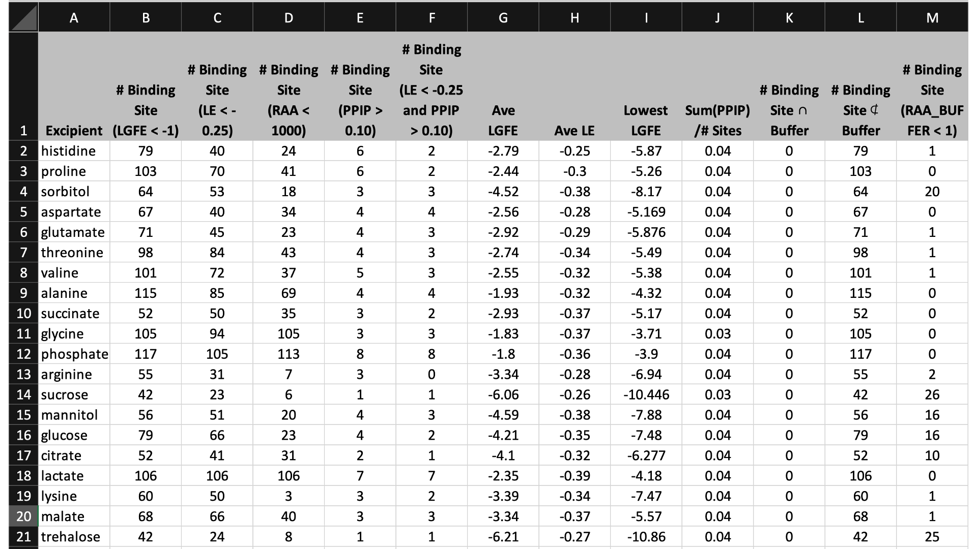
The contents of the columns are:
A: The excipient.
B: The number of binding sites where the excipient binds with an Ligand Grid Free Energy (LGFE) < -1 kcal/mol. LGFE approximates the binding affinity.
C: The number of binding sites where the excipient Ligand Efficiency (LE) < -0.25 kcal/mol. LE provides a metric of the binding affinity normalized for molecular size. LE = LGFE / N_heavy_atom, where N_heavy_atom is the number of non-hydrogen atoms in the excipient.
D: The number of binding sites found with a Relative Affinity Analysis metric (RAA) < 1000. RAA indicates the number of “strong” binding sites accessible to each molecule. The RAA is a ratio of dissociation constants (Kd’s), where the numerator is the Kd for the excipient at a given pocket and the denominator is the Kd for the best-scoring (highest affinity) binding pose for that excipient across the entire protein. Kd is computed from LGFE, where LGFE is taken to be the free energy.
E: The number of binding sites with a sum of PPI preference for residues in the binding site (PPIP) > 0.10. A high PPIP value for a binding site suggests that site is more likely to contribute to a PPI.
F: The number of binding sites having both LE < -0.25 kcal/mol and PPIP > 0.10.
G: The average LGFE for the excipient.
H: The average LE for the excipient.
I: The LGFE for the best-scoring (highest affinity) pose of the excipient.
J: Sum(PPIP)/# sites is the sum of the PPIP values for all of the binding sites in column B divided by the value of column B. This gives an average PPIP value computed accross the excipient-favored binding sites.
K: The number of binding sites that overlap with buffer binding sites. If no buffer was specified, this number will be zero. If all excipient binding sites are also capable of binding buffer, this number will be equal to the value in column B.
L: The number of excipient binding sites that are not also buffer binding sites. If no buffer was specified, this number will be equal to the value in column B.
M: The number of binding sites where the excipient has a higher binding affinity (i.e, lower Kd or, equivalently, more negative LGFE) than the buffer at that site. In otherwords, the number of binding sites where this excipient will out-compete buffer for binding. If no buffer was specified, this computation is done relative to a hypotheical buffer with an LGFE of -4 kcal/mol.
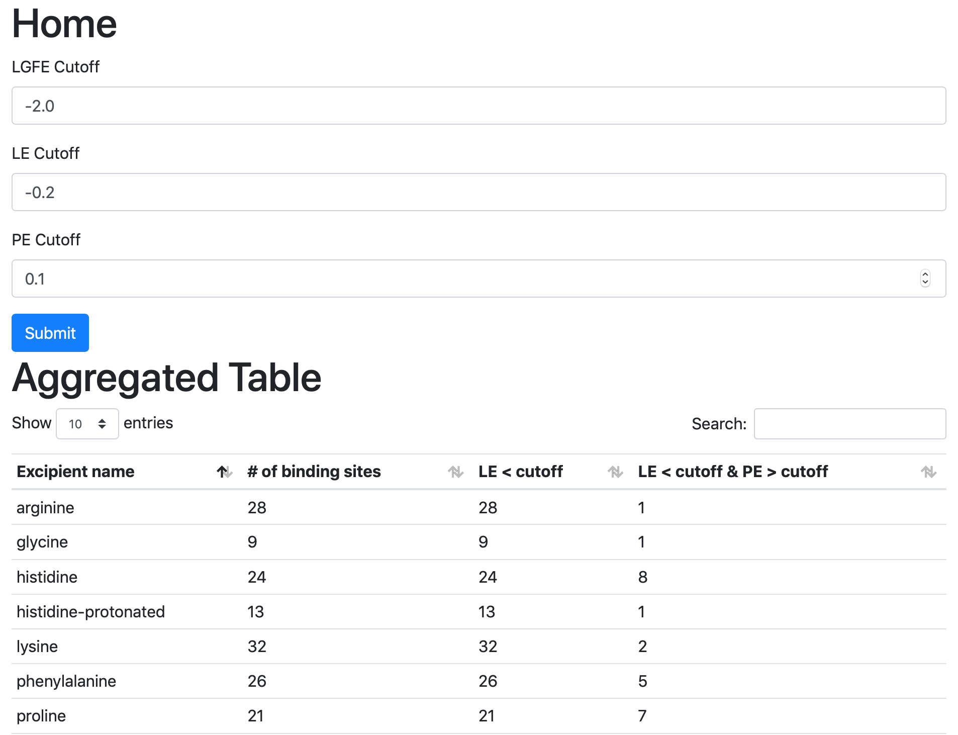
To proceed with the web view:
cd $WORKDIR/4_report.$job_id/view
sh run.sh
sh run.sh will print out a message like:
* Serving Flask app "main.py" (lazy loading)
* Environment: development
* Debug mode: on
* Running on http://0.0.0.0:5000/ (Press CTRL+C to quit)
* Restarting with stat
* Debugger is active!
* Debugger PIN: 222-574-256
Open a web browser and go to the URL displayed in the output (e.g., http://127.0.0.1:5000 or http://<IP address>:5000).
If you are running the web view from a remote server and if the server is behind a firewall, you may not able to directly access the web view. In this case, you can use a method called SSH port forwarding. This uses an SSH connection to the remote server to access the web view securely.
If you are using Linux, MacOS, or Linux subsystem on Windows as your desktop:
Open a terminal;
SSH to the remote server using the following example SSH command in the terminal;
ssh -L 5000:localhost:5000 username@servernameOpen a tab in the web browser, and navigate to
localhost:5000.
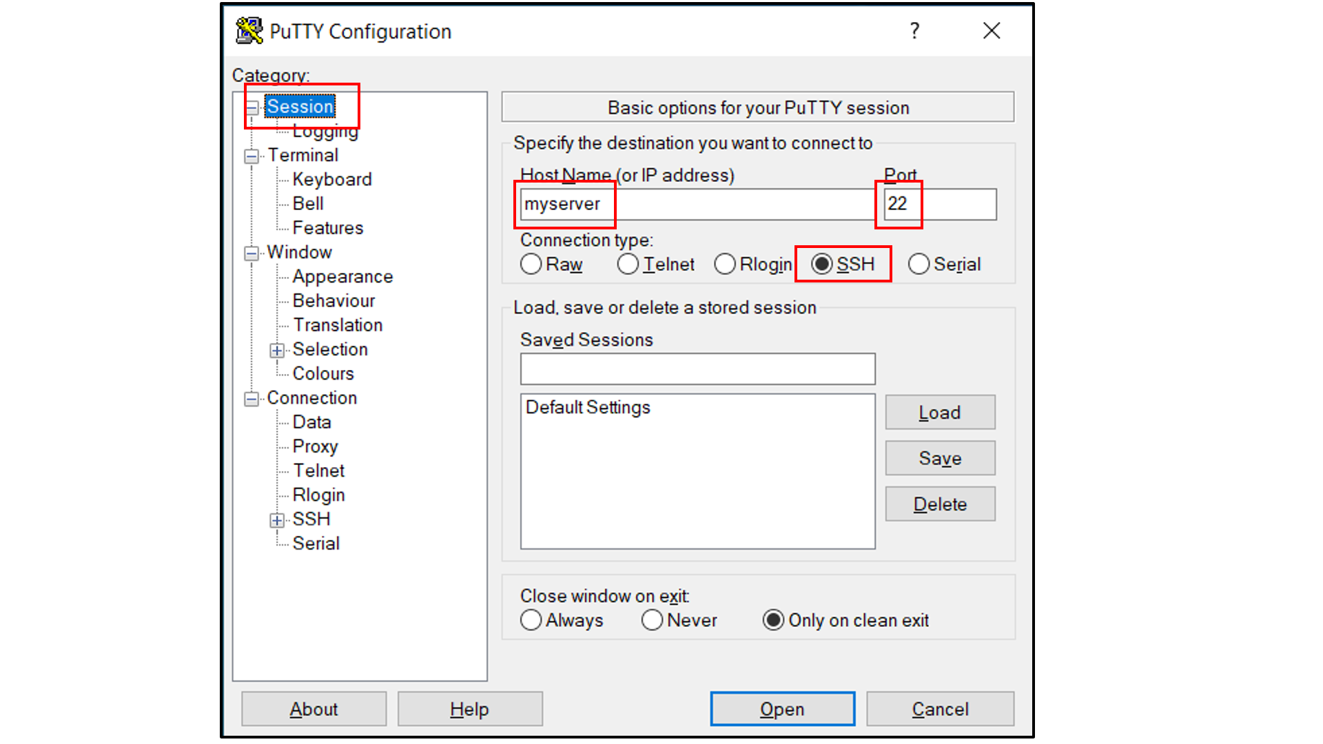
If you are using Windows as your desktop and and the PuTTY application for SSH access:
Open PuTTY
Select “Session”, and
Type in the target host name and port (default: 22);
Choose SSH as the connection type (default);
Select “Connection -> Data”, and
Type in your username as the auto-login username
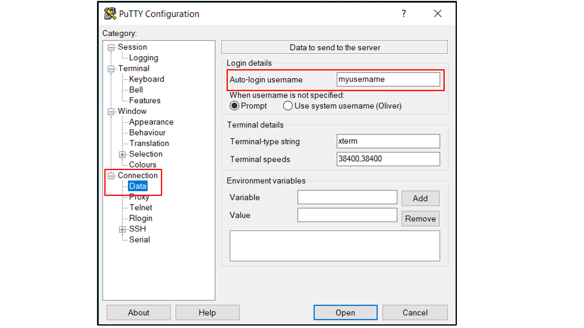
Select “Connection -> SSH -> Tunnels”, and
In “Source port”, type in
5000;In “Destination”, type in
localhost:5000;Click the “Add” button on the right side of “Source port” box;
Turn on the Local and Auto radio buttions (default) below the “Destination” box;
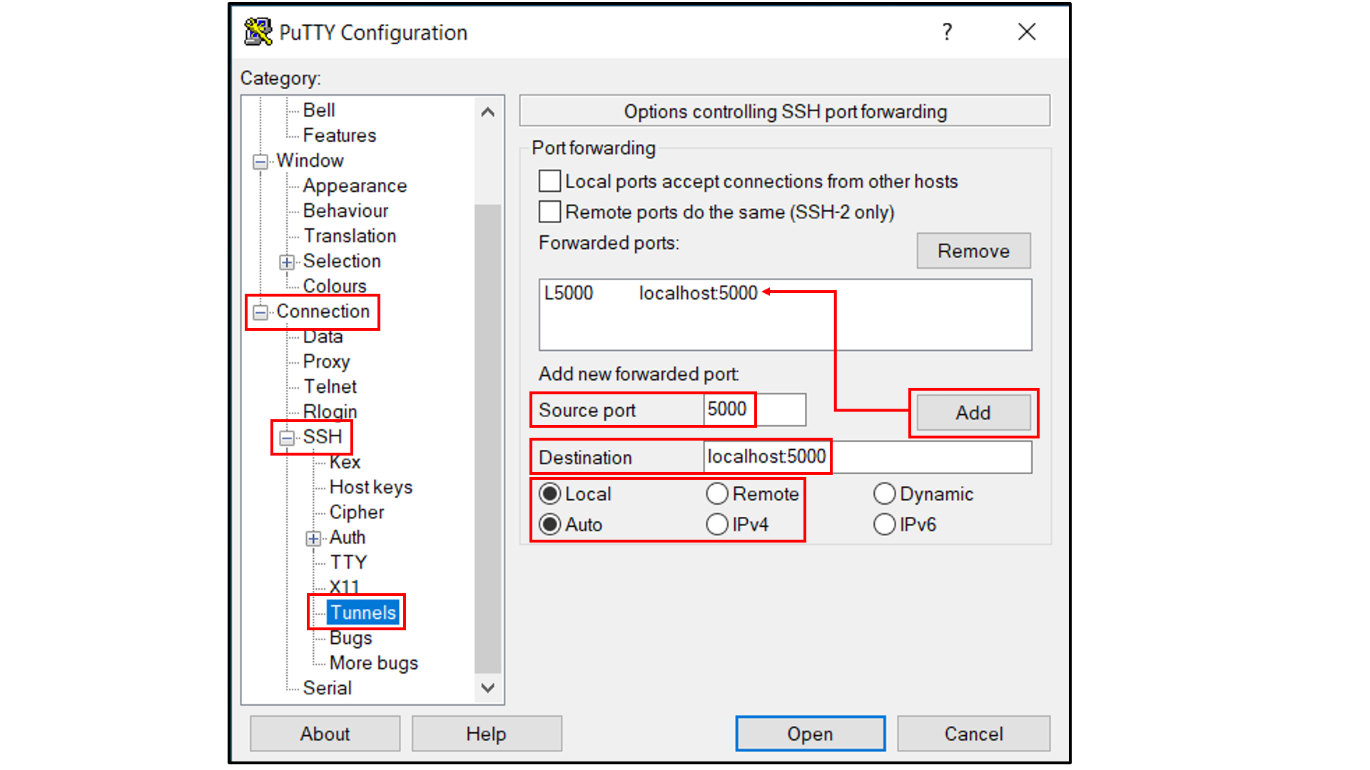
Select “Session”, and
Choose a name for the session;
Click the “Save” button to save the session with all your parameters;
Click “Open” to open a terminal to connect to your remote server.
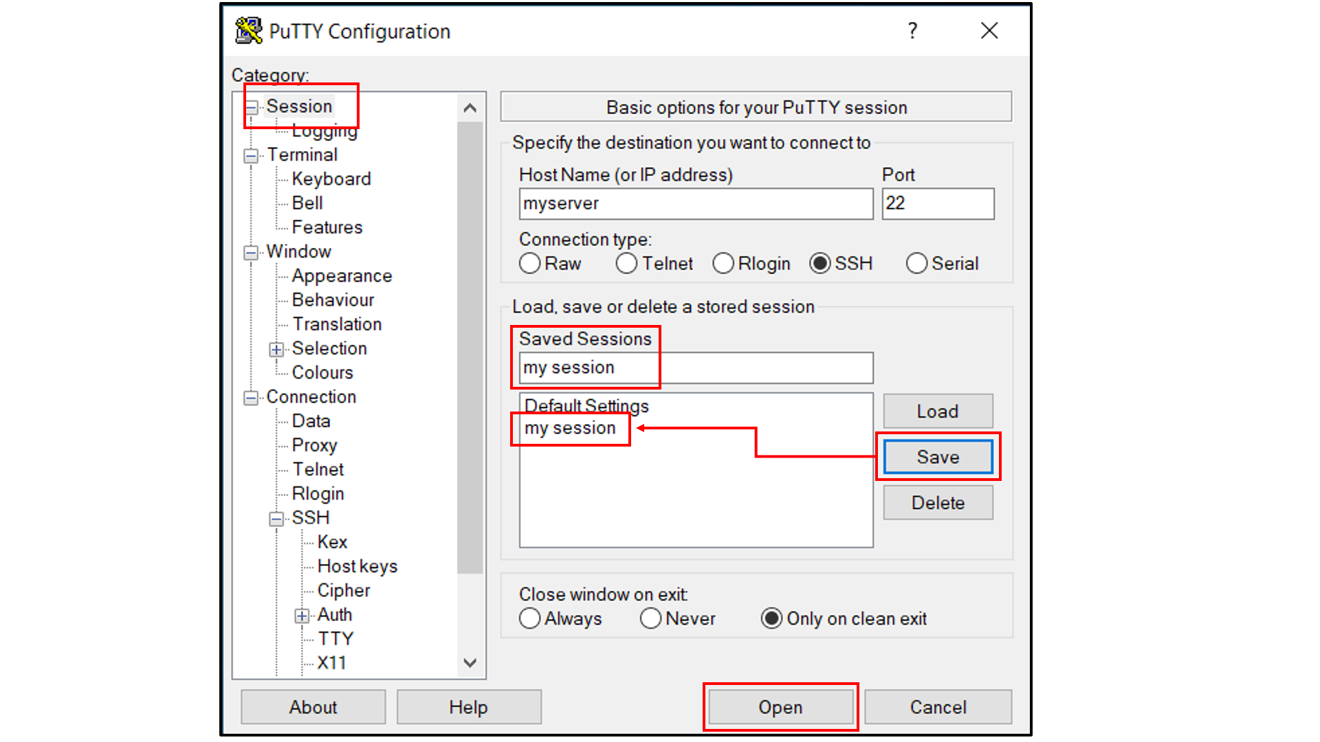
Open a tab in the web browser, and navigate to
localhost:5000.
Data interpretation
The data output from Step 4 can help connect experimental observables to the molecular details of protein-excipient interation. In doing so, these simulation data can help both rationalize known trends for existing data on excipients and suggest the choice of new excipients for additional testing. With regard to the former, the most straightforward approach is to compare available experimental data to the Step 4 output and note correlations:
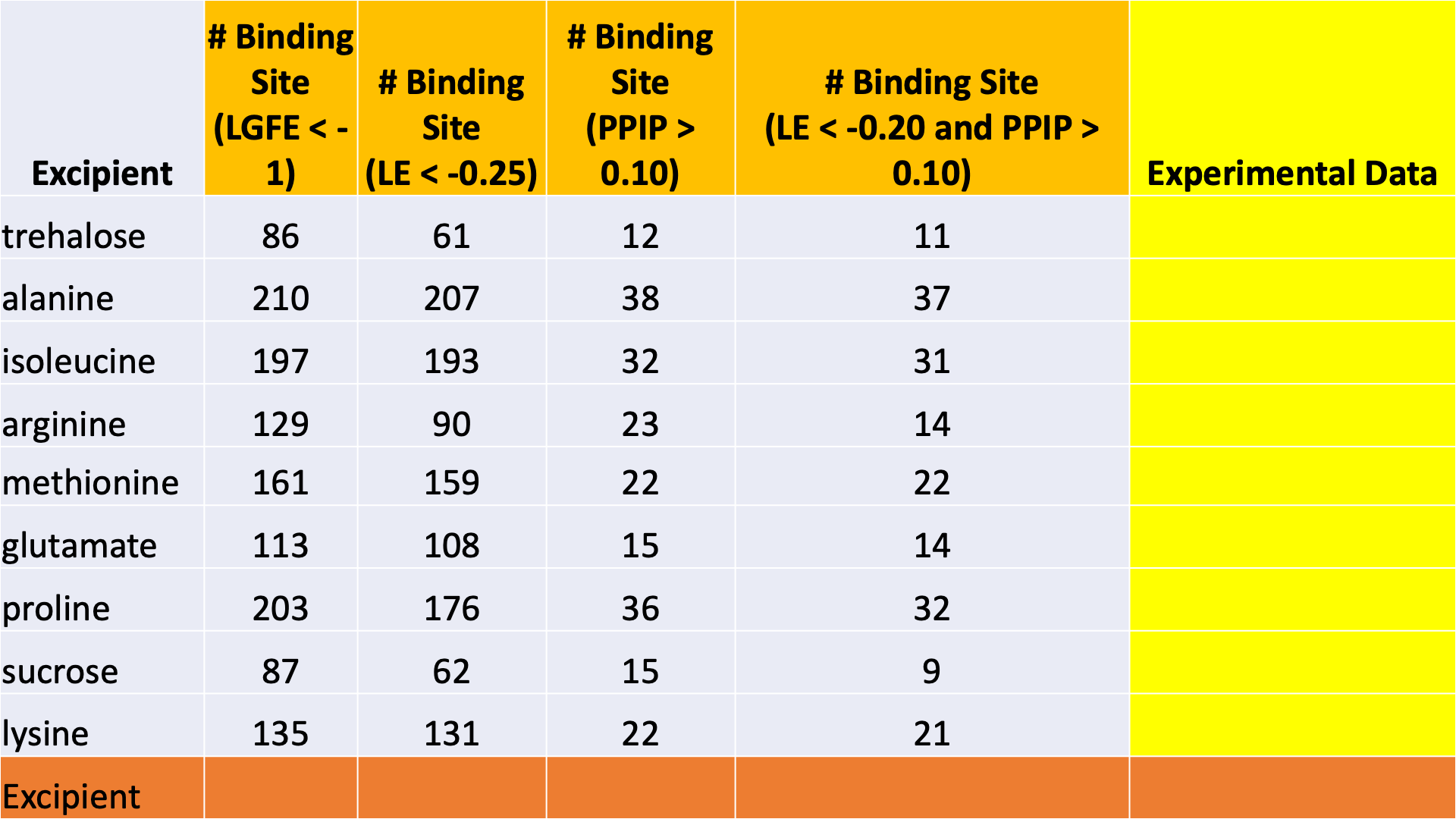
Please see [2] for a real-world example.
SilcsBio is currently developing methodology to compute relative occupancies of excipient binding sites for solutions containing more than one excipient. Please contact support@silcsbio.com for early access to this methodology and for additional help with data interpretation.
Visualizing SILCS FragMaps
Your SilcsBio software provides convenient ways to visualize SILCS
FragMaps generated during Step 1 of the SILCS-Biologics workflow using
your choice of MOE, PyMol, or VMD. FragMaps will be stored in
$WORKDIR/1_fragmap.$job_id/fab/silcs_fragmaps_fab.
Please see Visualizing FragMaps with external software (MOE, PyMol, VMD) for detailed instructions.
Visualizing SILCS-PPI results
SILCS-Biologics Step 2 SILCS-PPI results can be viewed using
molecular graphics software. For the purposes of SILCS-PPI, one protein
is considered the “receptor” and the other the “ligand”. In the current
use case with only one input protein domain, prot1=fab.pdb,
fab.pdb data are used for both the “receptor” and the “ligand”. For
the purpose of SILCS-PPI, the ligand protein is docked to the receptor
protein by comprehensively sampling locations and orientations of the
ligand protein relative to the receptor protein. The relative locations
and orientations are scored based on the overlap of the ligand
functional groups and the receptor protein SILCS FragMaps (computed in
Step 1). The docked poses of the ligand are then clustered as part of
SILCS-PPI.
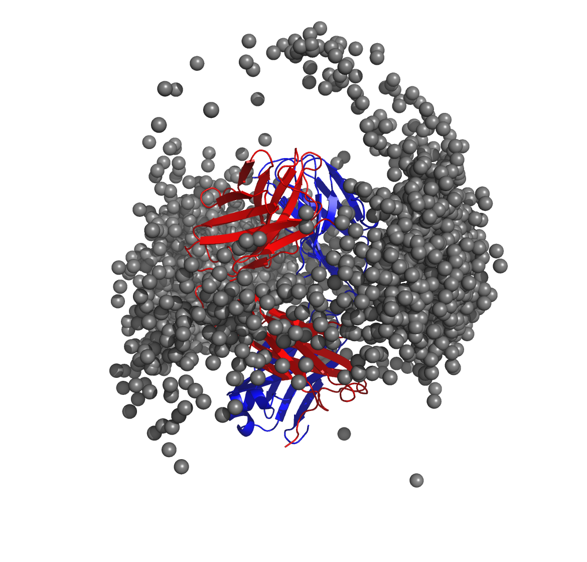
The $WORKDIR/2_ppi.$job_id/fab_fab/3_ppi/receptor_clusters.pdb file
contains the receptor protein structure and the cluster centroids. The
cluster centroids in this file all have the same chain name, Z.
Below is a molecular graphics image of receptor_clusters.pdb, with
the receptor protein shown as ribbons and the cluster centroids as
spheres. The CDR loops of the Fab are pointing to the top of the image,
heavy chain amino acids are in red, light chain amino acids are in blue,
and cluster centroids in gray.
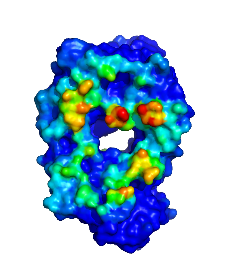
$WORKDIR/2_ppi.$job_id/fab_fab/3_ppi/receptor_surf_contact.pdb
contains PPI propensity values mapped onto the receptor protein and
recorded in the B-factor column, which provides an easy way to visualize
which residues are most at risk for contributing to PPI, and, therefore,
to aggregation of the biologic in its native (folded) state:
Use Case 2. Running SILCS-Biologics for a protein with two domains
In this example, we start with a full-length structure of a hypothetical
protein, fullpdb.pdb, with two independent domains, domain X and
Y. To begin, you must create two input protein domain files
corresponding to each domain.
To do so, simply make two copies of fullpdb.pdb and name one
protx.pdb and the other proty.pdb. Then, edit protx.pdb and
delete the amino acids corresponding to the domain Y. Repeat the same
process for proty.pdb; edit proty.pdb and delete the amino acids
corresponding to the domain X. Make sure that there is no overlap
between the amino acids contained in protx.pdb and proty.pdb. In
general, all amino acids in fullpdb.pdb should be accounted for by
the combination of protx.pdb and proty.pdb; however, if long
flexible peptide connects protx.pdb to proty.pdb, the amino
acids in that peptide region can be excluded from protx.pdb and
proty.pdb for computational expediency with likely minimal impact on
the final results.
$SILCSBIODIR/silcs-biologics/silcs-biologics \
    step=1*2*3*4* \
    prot1=protx.pdb \
    prot2=proty.pdb \
    fullpdb=fullpdb.pdb
Note that there are now two additional input parameters relative to Use
Case 1: prot2=proty.pdb and fullpdb=fullpdb.pdb. The addition of
prot2= indicates a second input protein domain must be considered
and the addition of fullpdb= provides a reference structure for
collating PPI contact data as well as for excluding surface-exposed
amino acids in protx.pdb and proty.pdb that are in fact buried
in the context of fullpdb.pdb. This latter point is important for
both the SILCS-PPI and SILCS-Hotspots analysis to ensure that buried
amino acids in full.pdb are not incorrectly noted as either
contributing to PPI or having hotspots. Both of the additional input
parameters, prot2= and fullpdb=, are required.
Note
If you do not have full-length structure, but only have the
structures of each domains, then you will have to create the
full-length structure using other molecular modeling tools (such as
homology modeling software or simple alignment to known full-length
homologous crystal structure) to utilize this workflow. Save the
resulting full-length structure as fullpdb.pdb and create
protx.pdb and proty.pdb as described at the beginning of this
example.
As with the Use Case 1, you may specify a directory containing a custom
set of excipients by adding molsdir=<path to my excipient directory>
and/or rank the excipients relative to a buffer molecule by adding
buffer=<path to my buffer mol2 file>.
Use Case 3. Running SILCS-Biologics for a protein with three domains
A complete antibody molecule is a large protein, consisting of ~1300 amino acids. Additionally, for the purposes of molecular dynamics simulations, it requires a very large simulation box for solvation because of its extended Y-shaped conformation. Splitting it into three domains, specifically its two Fab regions and the one Fc region, makes the molecular dynamics-based SILCS simulations substantially more computationally tractable. Not only are the individual domains each ~1/3 the size of the full antibody, but also, when considered individually, the Fab and Fc regions are very compact and therefore can be simulated inside relatively small simulation boxes to achieve appropriate solvation.
We start with a full-length structure of the antibody, antibody.pdb.
From this file, you must create three input protein domain files
corresponding to the two Fab regions and the one Fc region, which we
will call faba.pdb, fabb.pdb, and fc.pdb, respectively. Make
three copies of antibody.pdb and name one faba.pdb, another
fabb.pdb, and the third fc.pdb. Then, edit faba.pdb and
delete the amino acids corresponding to the second Fab and the Fc
regions. Edit fabb.pdb and delete the amino acids corresponding to
the first Fab and the Fc region. And edit fc.pdb and delete the
amino acids corresponding to the first Fab and the second Fab regions.
Make sure that there is no overlap between the amino acids contained in
faba.pdb, fabb.pdb and fc.pdb.
In general, all amino acids in fullpdb.pdb should be accounted for
by the combination of faba.pdb, fabb.pdb, and fc.pdb;
however, if long flexible peptide connects faba.pdb, fabb.pdb,
and/or fc.pdb, the amino acids in that peptide region can be
excluded from faba.pdb, fabb.pdb, and fc.pdb for
computational expediency with likely minimal impact on the final
results. An example can be found in $SILCSBIODIR/examples/nist_mab/
folder.
$SILCSBIODIR/silcs-biologics/silcs-biologics \
    step=1*2*3*4* \
    prot1=faba.pdb \
    prot2=fabb.pdb \
    prot3=fc.pdb \
    fullpdb=antibody.pdb
Note that there is one additional required input parameter relative to
Use Case 2: prot3=fc.pdb. The addition of prot3= indicates a
third input protein domain will be considered. As with Use Case 2,
fullpdb= indicates a reference structure for collating PPI contact
data as well as for excluding surface-exposed amino acids in individual
input protein domains that are in fact buried in the context of
antibody.pdb. Note that all of the input parameters in the above
example are required.
Note
If you do not have full-length antibody structure, but only have the structures of Fab and Fc domains, then you will have to create the full-length structure using other molecular modeling tools (such as homology modeling software.
Alternatively, you can align the domains onto other full-length IgG
structures (e.g., PDB:1HZH from RCSB database). Save the resulting
full-length structure as fullpdb.pdb and create faba.pdb,
fabb.pdb, and fc.pdb as described at the beginning of this
example.
As with the other use cases, you may specify a directory containing a
custom set of excipients by adding molsdir=<path to my excipient
directory> and/or rank the excipients relative to a buffer molecule by
adding buffer=<path to my buffer mol2 file>.
Running the workflow one step at a time
silcs-biologics can be used to run the SILCS-Biologics workflow in a
stepwise fashion, with step=1* requesting only the SILCS simulations
be run, step=2* requesting SILCS-PPI be run, step=3* requesting
SILCS-Hotspots be run, and step=4* requesting processing of data
from the prior steps and generation of the final report. Finer control
at the level of the smaller substeps can also be requested, as detailed
in the following example.
Stepwise Use Case 1. One input protein domain
In this example, we use fab.pdb as the input protein domain. You can
find this file in $SILCSBIODIR/examples/biologics/nist_fab/.
Step 1: Run SILCS and generate FragMaps
You can run all the substeps of Step 1 automatically:
$SILCSBIODIR/silcs-biologics/silcs-biologics \
    step=1* \
    prot1=fab.pdb \
    job_id=try01
The
job_id=parameter is used to group together job inputs and outputs from different steps/substeps. Therefore, when usingsilcs-biologicsin a stepwise fashion, you will need to provide the same value for this parameter across all steps/substeps for the system you are modeling.Alternatively, you can run substep by substep:
Step 1a: Set up SILCS simulations
$SILCSBIODIR/silcs-biologics/silcs-biologics \
    step=1a \
    prot1=fab.pdb \
    job_id=try01
Step 1b: Run SILCS simulations
$SILCSBIODIR/silcs-biologics/silcs-biologics \
    step=1b \
    prot1=fab.pdb \
    job_id=try01
These SILCS simulations for
fab.pdbwill take 1 to 2 days on a cluster with 10 GPU-enabled compute nodes. If the simulation jobs fail due to external factors such as a power outage, server maintenance, etc., you can use the exact same command to resume the SILCS jobs from the point where they failed (as opposed to needing to restart them from the very beginning).Step 1c: Generate SILCS FragMaps
$SILCSBIODIR/silcs-biologics/silcs-biologics \
    step=1c \
    prot1=fab.pdb \
    job_id=try01
Step 2: Run SILCS-PPI
To continue with Step 2 using your outputs from Step 1, run your commands in the same directory where you ran your Step 1 commands and use the same
$job_idyou used for Step 1.You can run all the substeps of Step 2 automatically:
$SILCSBIODIR/silcs-biologics/silcs-biologics \
    step=2* \
    prot1=fab.pdb \
    job_id=try01
Alternatively, you can run each substep by using the following commands:
Sub-step 2a: Run SILCS-PPI jobs
$SILCSBIODIR/silcs-biologics/silcs-biologics step=2a \
    prot1=fab.pdb \
    job_id=try01
Sub-step 2b: Collect PPI results
$SILCSBIODIR/silcs-biologics/silcs-biologics \
    step=2b \
    prot1=fab.pdb \
    job_id=try01
Step 3: Run SILCS-Hotspots
To continue with Step 3 using your outputs from Step 2, run your commands in the same directory where you ran your Step 2 commands and use the same
$job_idyou used for Step 1 and Step 2.As described previously in Running the complete workflow with a single command, you can specify a custom set of excipient molecules using the optional
molsdir=parameter.You can run all the substeps of Step 3 automatically:
$SILCSBIODIR/silcs-biologics/silcs-biologics \
    step=3* \
    prot1=fab.pdb \
    job_id=try01
Alternatively, you can run each substep by using the following commands:
Step 3a: Run excipient docking
$SILCSBIODIR/silcs-biologics/silcs-biologics \
    step=3a \
    prot1=fab.pdb \
    job_id=try01
Step 3b: Cluster the hotspots
$SILCSBIODIR/silcs-biologics/silcs-biologics \
    step=3b \
    prot1=fab.pdb \
    job_id=try01
Step 4: Collate and analyze data from prior steps and generate report
The SILCS-Biologics data can be processed into a web report or a spreadsheet report. As described previously in Running the complete workflow with a single command, you can specify a buffer molecule that will be used as a reference for ranking of the excipients using the optional
buffer=parameter.Generate a web report
$SILCSBIODIR/silcs-biologics/silcs-biologics
    step=4a \
    prot1=fab.pdb \
    job_id=try01
Run step 4b only (Spreadsheet_Report)
$SILCSBIODIR/silcs-biologics/silcs-biologics
    step=4b \
    prot1=fab.pdb \
    job_id=try01
Stepwise Use Case 2. Two input protein domains
Follow the instructions for Use Case 1. Running SILCS-Biologics with a single protein domain, and,
in addition to prot1=, provide values for prot2=
and fullpdb=.
Stepwise Use Case 3. Three input protein domains
Follow the instructions for Use Case 1. Running SILCS-Biologics with a single protein domain, and,
in addition to prot1=, provide values for prot2=, prot3=,
and fullpdb=.
Re-running a system with a different set of excipients
If, after having run the SILCS-Biologics workflow, you decide you would
like results for additional excipients, you can simply reuse your
existing results from Step 1 (SILCS) and Step 2 (SILCS-PPI) without
re-running these two steps. To do so, you will need to use a new
$job_id for the new set of excipients. Let us assume your original
simulations were in $WORKDIR and had the $job_id value
try01. After initially completing the SILCS-Biologics workflow, you
would have the following directories:
$WORKDIR/1_fragmap.try01
$WORKDIR/2_ppi.try01
$WORKDIR/3_excipients.try01
$WORKDIR/4_report.try01
To re-use your existing SILCS FragMap and SILCS-PPI data, copy the contents
of their respective directories and associate the new directories with a
new $job_id, try02:
cd $WORKDIR
cp -r 1_fragmap.try01 1_fragmap.try02
cp -r 2_ppi.try01 2_ppi.try02
Tip
To save disk space, you may create symbolic links to instead of making copies of your existing data.
cd $WORKDIR
ln -s 1_fragmap.try01 1_fragmap.try02
ln -s 2_ppi.try01 2_ppi.try02
However, be mindful that with symbolic links any changes you make to
1_fragmap.try02 or to 2_ppi.try02 (including deleting files)
will also be made to 1_fragmap.try01 and 2_ppi.try01.
Therefore, we strongly recommend you use cp -r instead of ln
-s if you have disk space available.
Now, re-run Step 3 and Step 4 using job_id=try02:
$SILCSBIODIR/silcs-biologics/silcs-biologics
    step=3*4* \
    prot1=fab.pdb \
    molsdir=my_excipients_new
The above command will use excipient files contained in
$WORKDIR/my_excipients_new for running the SILCS-Hotspots
calculations and creating reports, and these results will be in the new
directories 3_excipients.try02 and 4_report.try02, respectively.
If you like, you can also add the buffer= option. This same approach
will also work for two or three input protein domains. Simply use the
prot2=, prot3=, and fullpdb= options as you used for your
initial job_id=try01 run through the SILCS-Biologics workflow.
Conserving computing resources for antibody simulations
The most straightforward way to apply SILCS-Biologics to an antibody is
to follow the directions for Use Case 3. Running SILCS-Biologics for a protein with three domains, and
we strongly recommend that new users use that approach. That said, it is
possible to conserve computing resources by taking advantage of the fact
that for a normal antibody (i.e., not a bi-specific antibody), the amino
acid composition of the two Fab regions is identical. In other words,
the amino acid sequence in faba.pdb is identical to fabb.pdb,
and their structures are therefore also very similar. As such, a single
set of SILCS FragMaps can be used for both Fab regions instead of
computing FragMaps independently for both faba.pdb and for
fabb.pdb.
Similar to Use Case 3. Running SILCS-Biologics for a protein with three domains, you will have to create
faba.pdb, fabb.pdb, and fc.pdb files from the full-length
antibody structure, fulllength.pdb before we begin.
Generate FragMaps for one of the Fab domain using the following command.
$SILCSBIODIR/silcs-biologics/silcs-biologics \
    step=1* \
    prot1=faba.pdb \
    job_id=try01
Generate FragMaps for
Fcdomain using the following command (This can be done in parallel with the step 1).$SILCSBIODIR/silcs-biologics/silcs-biologics \ step=1* \ prot1=fc.pdb \ job_id=try01Generate FragMaps for another Fab domain using the following command.
python $SILCSBIODIR/utils/python/reorient_maps.py faba.pdb fabb.pdb \
    1_fragmap.try01/faba/silcs_fragmaps_faba \
    --outdir 1_fragmap.try01/fabb/silcs_fragmaps_fabb/maps
Continue running the remaining steps from 2 to 4 using the following command.
$SILCSBIODIR/silcs-biologics/silcs-biologics \
    step=2*3*4* \
    prot1=faba.pdb \
    prot2=fabb.pdb \
    prot3=fc.pdb \
    fullpdb=antibody.pdb
SILCS-Biologics directory structure
silcs-biologics creates the below directories in $WORKDIR.
By default, $WORKDIR is the directory in which silcs-biologics
was run. Otherwise, $WORKDIR is determined by the parameter passed to
silcs-biologics through the command line option workdir=.
Step 1 SILCS FragMap results will be in 1_fragmap.$job_id/,
                                      |>>> 1_setup
                      |>>> $prot1 >>> |>>> 2a_run_gcmd
                      |               |>>> 2b_gen_maps
                      |               |>>> silcs_fragmaps_$prot1
1_fragmap.$job_id >>> |>>> $prot2 ...
                      |>>> $prot3 ...
Step 2 SILCS-PPI results will be in 1_ppi.$job_id/,
                                         |>>> maps1
                  |>>> $prot1_$prot1 >>> |>>> maps2
                  |                      |>>> 3_ppi
2_ppi.$job_id >>> |>>> $prot1_$prot2 ...
                  |>>> $prot1_$prot3 ...
                  |>>> $prot2_$prot1 ...
                  |>>> $prot2_$prot2 ...
                  |>>> $prot2_$prot3 ...
                  |>>> $prot3_$prot1 ...
                  |>>> $prot3_$prot2 ...
                  |>>> $prot3_$prot3 ...
Step 3 SILCS-Hotspots excipient docking results will be in
3_excipients.$job_id/,
                          |>>> mols
                          |>>> $prot1 >>> 4_hotspots >>> ***
3_excipients.$job_id >>>  |>>> $prot2 ...
                          |>>> $prot3 ...
and Step 4 reporting will be in 4_report.$job_id,
4_report.$job_id