SILCS-Pharm: Receptor-Based Pharmacophore Models from FragMaps
Background
Three-dimensional (3-D) pharmacophore models (also called “hypotheses”) offer an intuitive and powerful approach for virtual screening (VS). 3-D pharmacophore VS works by searching for matches between the 3-D pattern of functional groups constituting a pharmacophore model and the 3-D arrangement of functional groups in ligand conformers in a virtual database. Ligands having conformers that closely match the pharmacophore model are considered hits. Traditionally, 3-D pharmacophore models were developed using experimental knowledge of the binding poses for ligands to a receptor. This is in contrast to energy function-based VS (“docking”). An advantage of docking approaches was that they only require experimental knowledge of the receptor structure, and not of bound ligands. However, it is possible to develop pharmacophore models using only the receptor structure. One means to generate such receptor-based pharmacophore models is with data from SILCS simulations.
SILCS-Pharm converts Grid Free Energy (GFE) FragMaps into 3-D pharmacorphore models. GFE FragMaps from SILCS simulations are used as inputs for the four-step SILCS-Pharm process:
voxel selection;
voxel clustering and FragMap feature generation;
FragMap feature to pharmacophore feature conversion;
generation of a pharmacophore model for virtual screening (VS).
Here, “feature” refers to the identity and location of a chemical functional group and “pharmacophore model” is a collection of pharmacophore features.
FragMap generation from SILCS MD entails partitioning 3-D space into uniform cubic voxels and enumerating fragment binding probabilities for each voxel. The voxels are retained during Boltzmann-inversion of probabilities to create GFE FragMaps. As the GFE voxel value represents the binding strength of a functional group at that specific location on the protein surface, the first step identifies the most favorable interactions based on a particular GFE cutoff value. In the second step, clustering is performed to group adjacent voxels, with each unique cluster becoming a FragMap feature. In the third step, the FragMap features are classified and converted into pharmacophore features. Finally, the pharmacophore features are prioritized using Feature GFE (FGFE) scores to create a SILCS 3-D pharmacophore model [8]. In the current scheme, the program searches through five FragMap types: Generic Apolar, Generic Donor, Generic Acceptor, Methylammonium N, and Acetate O. Additionally, instead of using a rigidly-defined protein surface to determine regions that ligands cannot sample because of protein volume occlusion, the SILCS Exclusion Map is used. The Exclusion Map has been validated to be a better alternative to more traditional representations of the occluded volume of the protein, and it takes protein flexibility into account in an explicit way.
Running SILCS-Pharm
Running SILCS-Pharm from the SilcsBio GUI
Select New SILCS-Pharm project from the Home page.
Enter a project name and select your remote server. On the remote server, select the “Project Location” directory. Output files will be placed in a subdirectory
5_pharm/in the Project Direcory. Select the “FragMap Location,” which is where the FragMaps from the prior SILCS run are located on the server. Likewise, select the “Protein PDB File,” which was the input PDB file for the SILCS run.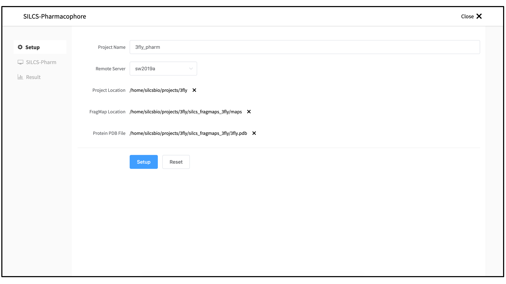
Once all information is entered correctly, press the “Setup” button at the bottom of the page. The GUI will contact the server, and a pop-over window will shows details of the communication with the server. When this is complete, press the green “Setup Successful” button to dismiss the pop-over window. The page will have updated to add “Pharmacophore Search” to the list of information. Click the “Select Pocket” button on the right-hand side of the window.
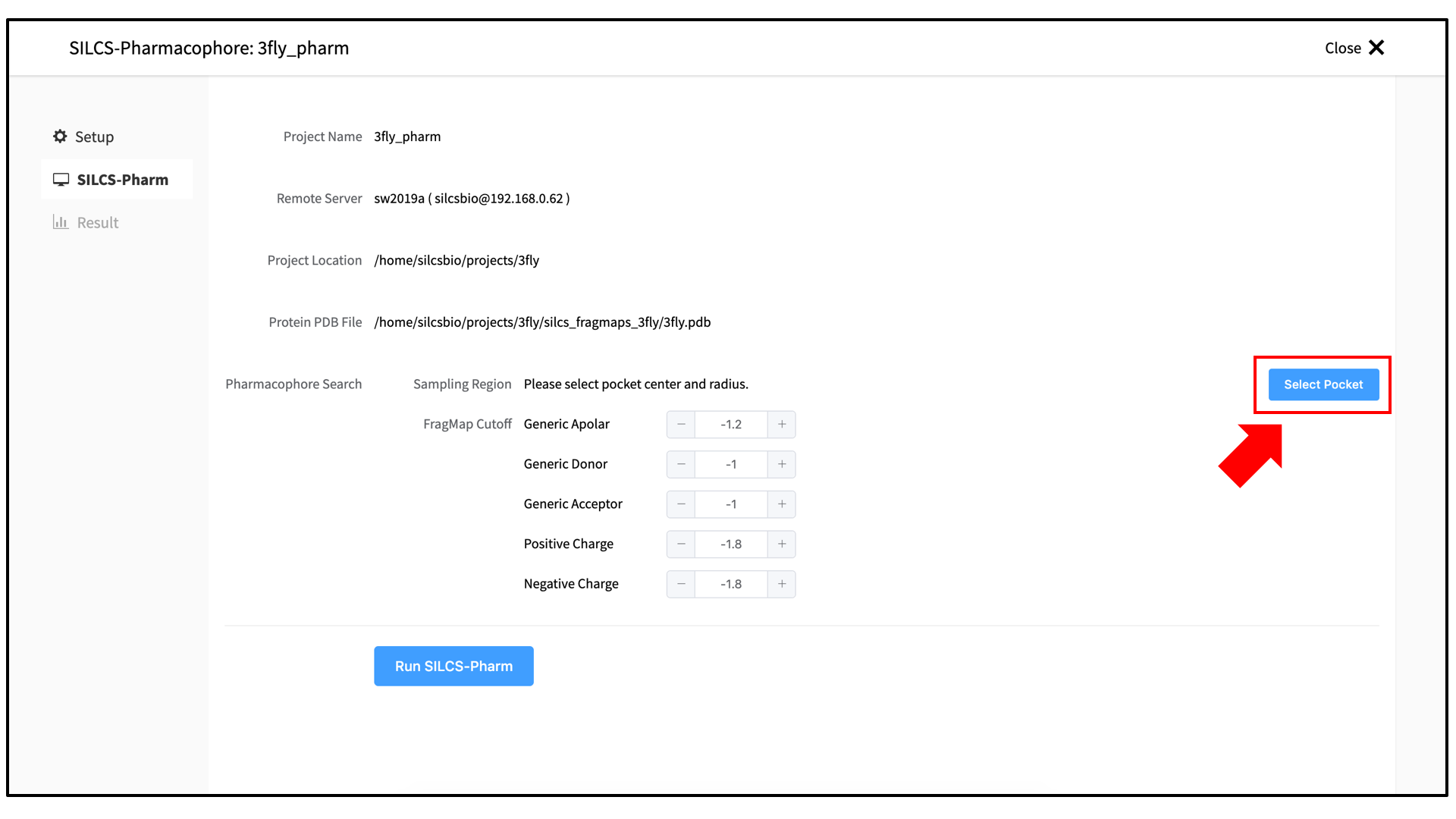
The GUI will now be showing the protein molecular graphic in the center pane. On the right-hand side, select the “Pocket” tab. From this tab, you can define the pocket center based on the center-of-geometry of a ligand pose (“Define Pocket using Ligand”), or a target residue selection (“Define Pocket using Selection”), or by directly entering an x, y, z coordinate (“Define Pocket by XYZ”). You will also need to choose a radius (default value “10”) to complete the definition of the spherical pocket. If it is difficult to see the spherical pocket definition in the center pane, click on the FragMap tab on the right-hand side and deselect the “Protein Surface” to hide the protein surface.
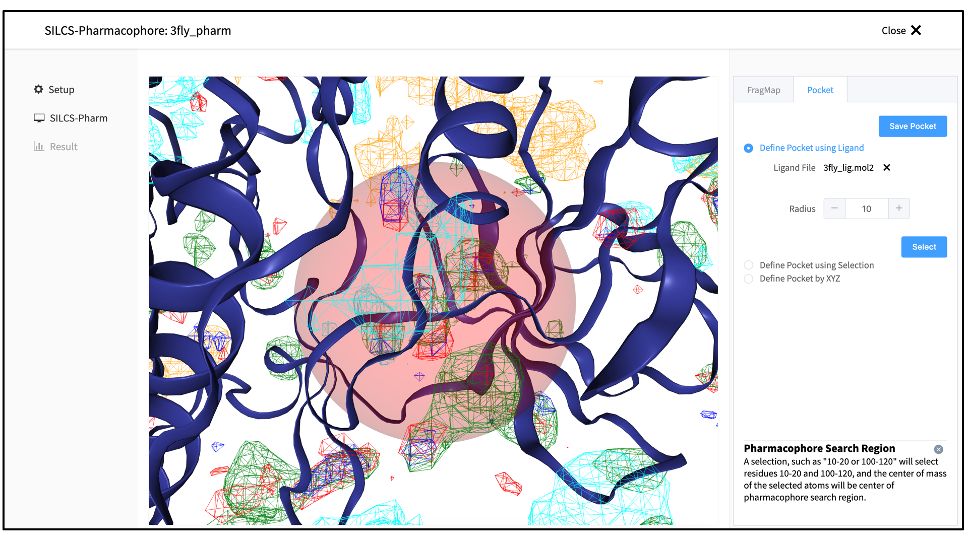
Click on the “Save Pocket” button to continue, and you will be returned to the previous screen, which now includes “Sampling Region” information consisting of the spherical pocket center and radius. You will also see default FragMap cutoff values listed for selection of FragMap densities for creation of pharmacophore features. You may adjust those values if you desire. Click on the “Run SILCS-Pharm” button to run the four-step SILCS-Pharm process.
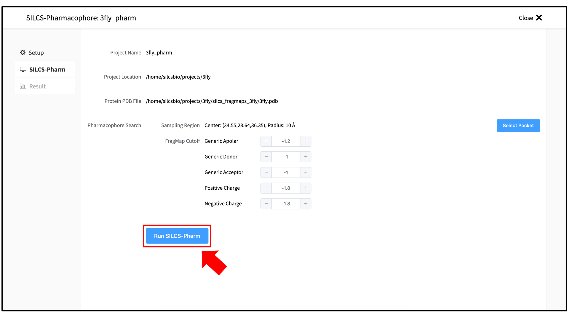
A pop-over window will appear and show output from the server, and the job will run to completion in a matter of seconds. Click on the “Search Finished” button. The GUI will proceed to download the SILCS-Pharm output from the server to the local computer for visualization. Click the green “Data Collection Finished” button to dismiss the pop-over window and reveal the molecular visualization of your pharmacophore features. You may wish to click on the “FragMap” tab in the right-hand panel and deselect the “Protein Surface” representation for easier viewing. The “Pharmacophore” tab will list all the pharmacophore features automatically generated from the FragMaps.
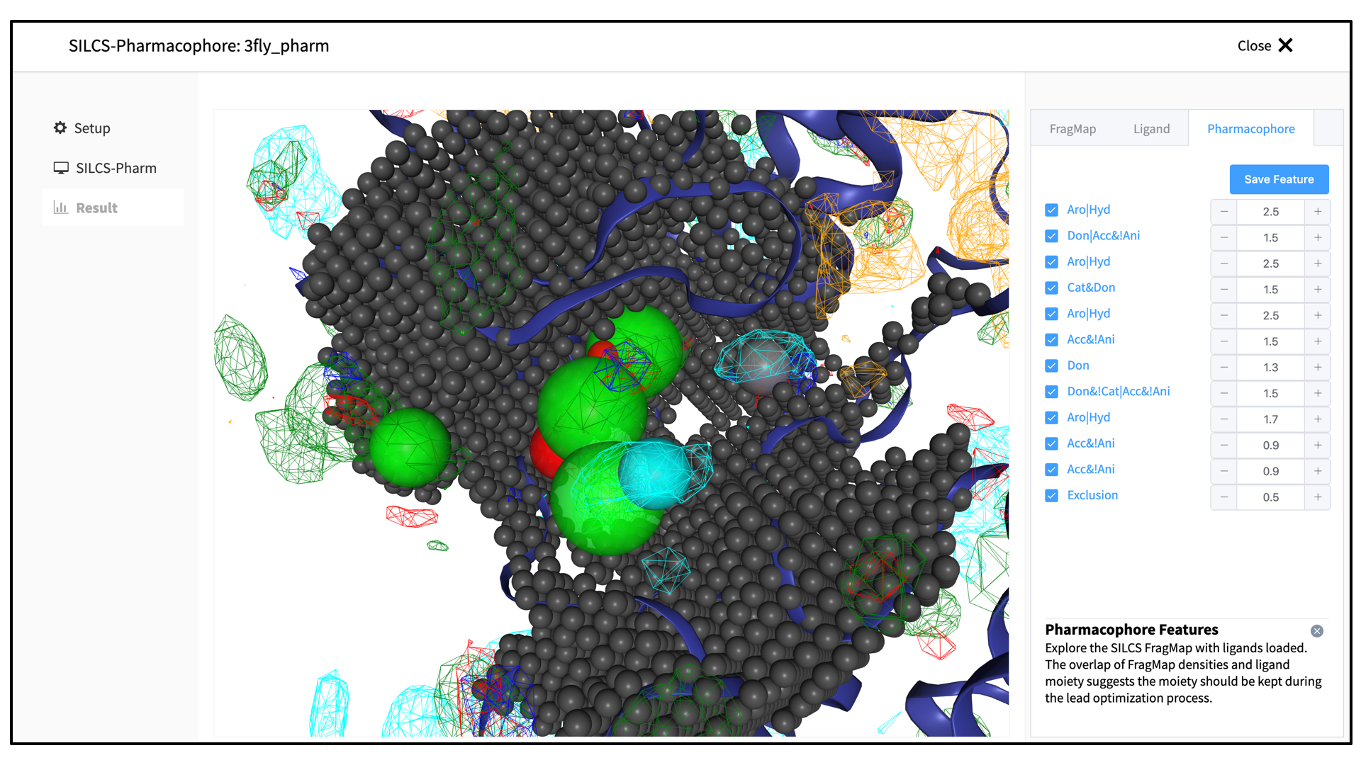
You may adjust the radii of the individual features or deselect them entirely. Once finished with pharmacophore feature selection and adjustment, click the “Save Feature” button. This will allow you to save your pharmacophore model containing your selected/adjusted features in
.ph4format on your local computer. By selecting/adjusting different subsets of the pharmacophore features, including the Exclusion Map, you may create multiple different pharmacophore models and save each one as a separate.ph4file. This capability allows for different pharmacophore model screens of a binding site. The resulting diverse hits from those screens can be combined and, for example, subjected to SILCS-MC Pose Refinement for rescoring.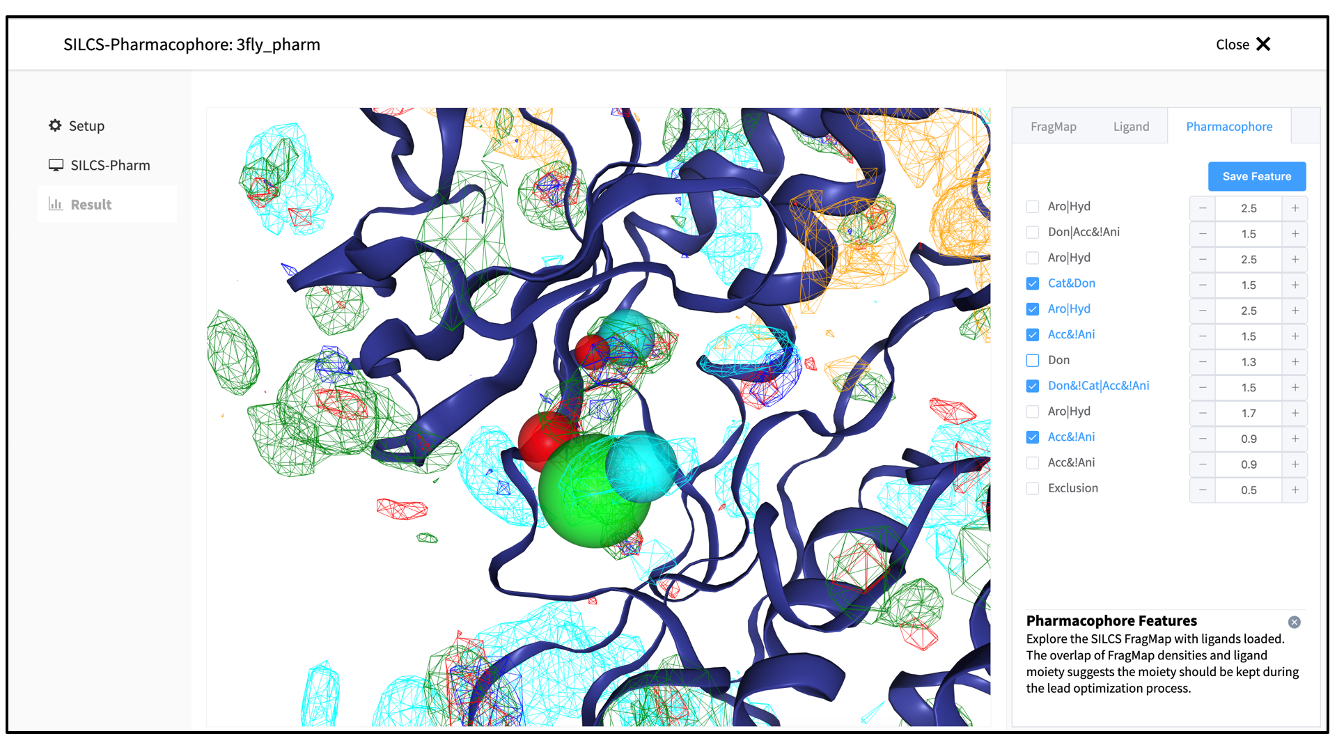
Running SILCS-Pharm from the command line interface
A single command line interface command performs the four-step SILCS-Pharm process:
${SILCSBIODIR}/silcs-pharm/1_calc_silcs_pharm prot=<prot pdb> center="x,y,z"
The input arguments are the PDB file used for the SILCS run and the absolute
position of the center of a 10 Å sphere to be used to define the boundaries of
the pharmacophore model. Two output files result from this command.
<prot>.keyf_<#features>.ph4 can be directly used for 3-D pharmacophore VS by
compatible programs (see below for generating Pharmer-compatible ph4 files).
<prot>_silcspharm_features.pdb provides output in PDB format for easy
visualization using standard molecular graphics packages. Running the command
with no arguments
${SILCSBIODIR}/silcs-pharm/1_calc_silcs_pharm
will list additional options. Along with the required arguments of prot=<prot
pdb> and center="x,y,z", the following additional options can be set:
FragMap directory path:
mapsdir=<location and name of directory containing FragMaps; default=2b_gen_maps>
By default, the program looks for FragMaps in the
2b_gen_mapsdirectory.Output directory path:
outputdir=<location and name of output directory; default=5_pharm>
By default, the program creates the directory
5_pharmand places all output files there.Radius:
radius=<default: 10>
By default, a radius of 10 Å centered at center=”x,y,z” is searched to generate pharmacophore features from the input FragMaps.
Generic Apolar FragMap cutoff:
apolar_cutoff=<default: -1.2>
By default, Generic Apolar FragMap voxels having a GFE value <= -1.2 kcal/mol are selected.
Generic Donor FragMap cutoff :
  hbdon_cutoff=<default: -1.0>

By default, Generic Donor FragMap voxels having a GFE value <= -1.0 kcal/mol
are selected.
Generic Acceptor FragMap cutoff :
hbacc_cutoff=<default: -1.0>
By default, Generic Acceptor FragMap voxels having a GFE value <= -1.0 kcal/mol are selected.
Methylammonium N FragMap cutoff :
mamn_cutoff=<default: -1.8>
By default, Methylammonium N FragMap FragMap voxels having a GFE value <= -1.8 kcal/mol are selected.
Acetate O FragMap cutoff :
aceo_cutoff=<default: -1.8>
By default, Acetate O FragMap FragMap voxels having a GFE value <= -1.8 kcal/mol are selected.
In addition to visualization, the output PDB file
<prot>_silcspharm_features.pdbcan be used for easy editing of the pharmacophore model. Using a text editor, modify/reduce the features in this file as desired and save the revised file as<prot>_silcspharm_features_revise.pdb. Using this revised PDB file and the original ph4 file<prot>.keyf_<#features>.ph4as input, create a new ph4 file with:${SILCSBIODIR}/programs/revise_ph4 <prot>.keyf_<#features>.ph4 <prot>_silcspharm_features_revise.pdbThe output of this command will be the revised ph4 file
<prot>.keyf_<#features>_revise.ph4. To create Pharmer-compatible ph4 output, add thepharmeroption:${SILCSBIODIR}/programs/revise_ph4 <prot>.keyf_<#features>.ph4 <prot>_silcspharm_features_revise.pdb pharmer
Example
The following example demonstrates use of SILCS-Pharm from the
command line interface to generate a
pharmacophore model for p38 MAP kinase. Input files, including FragMaps, are
provided in ${SILCSBIODIR}/examples/silcs/ (these same input files may
also be used for a trial run of SILCS-Pharm with the SilcsBio GUI).
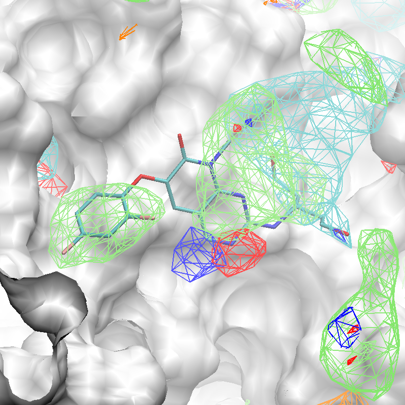
The x,y,z coordinates of the center of the complexed ligand are used to create a SILCS-Pharm 3-D pharmacophore model encompassing the ligand binding site (shown below). These coordinates define the center of the sphere within which FragMap voxels are searched and clustered to generate features.
Using the ligand center coordinates center="35.24, 27.48, 37.73", generate
the 3-D pharmacophore model with:
${SILCSBIODIR}/silcs-pharm/1_calc_silcs_pharm prot=3fly.pdb center="35.24,27.48,37.73" mapsdir=${SILCSBIODIR}/examples/silcs/silcs_fragmaps_3fly/maps
The command will complete after several seconds, and the output will note, “A
total of 13 features have been detected.” All output files will be in a new
subdirectory 5_pharm. Standard molecular graphics software can be used to
visualize the output file 3fly_silcspharm_features.pdb, which has one
ATOM entry for each of the 13 pharmacophore features:
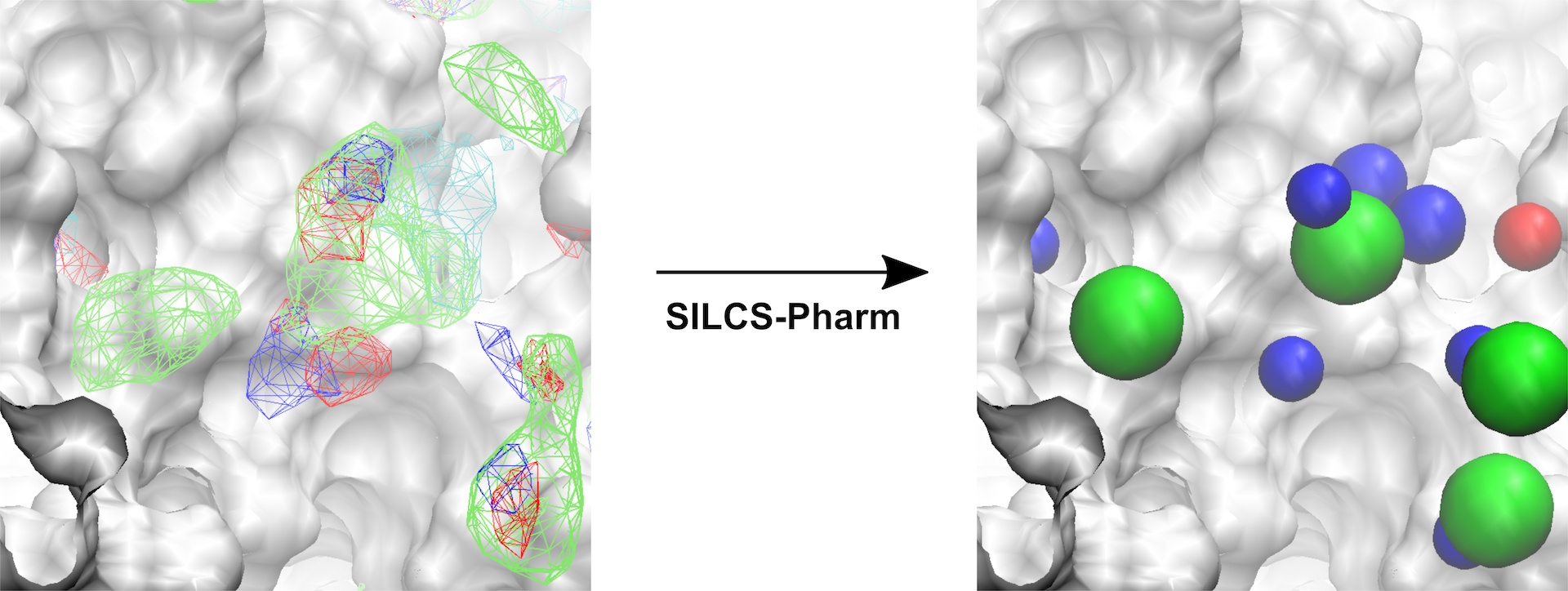
Fig. 4 Conversion of FragMaps (left) to SILCS pharmacophore features (right).
To modify/reduce the features, edit the output file
3fly_silcspharm_features.pdb and save it as
3fly_silcspharm_features_revise.pdb, then run
${SILCSBIODIR}/programs/revise_ph4:
${SILCSBIODIR}/programs/revise_ph4 3fly.keyf_13.ph4 3fly_silcspharm_features_revise.pdb
The output 3fly.keyf_13_revise.ph4 will reflect your revisions in
3fly_silcspharm_features_revise.pdb.
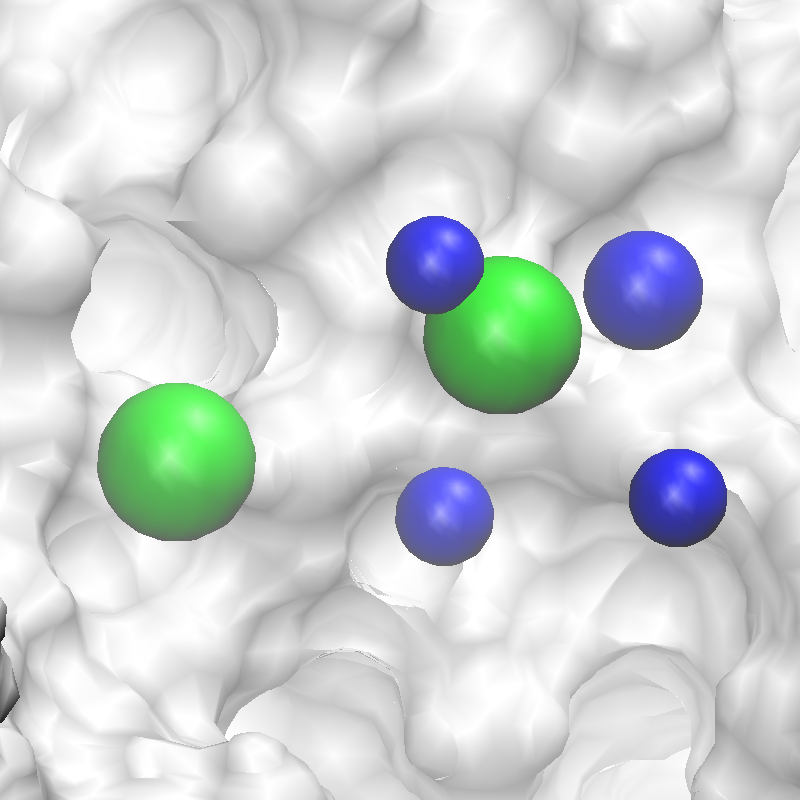
Fig. 5 Revised SILCS pharmacophore features.