SILCS: Site Identification by Ligand Competitive Saturation

Background

The design of small molecules that bind with optimal specificity and affinity to their biological targets, typically proteins, is based on the idea of complementarity between the functional groups in a small molecule and the binding site of the target. Traditional approaches to ligand identification and optimization often employ the one binding site/one ligand approach. While such an approach might be straightforward to implement, it is limited by the resource-intensive nature of screening and evaluating the affinity of large numbers of diverse molecules.

Functional group mapping approaches have emerged as an alternative, in which a series of maps for different classes of functional groups encompass the target surface to define the binding requirements of the target. Using these maps, medicinal chemists can focus their efforts on designing small molecules that best match the maps.

Site Identification by Ligand Competitive Saturation (SILCS) offers rigorous free energy evaluation of functional group affinity pattern for the entire 3D space in and around a protein [9]. The SILCS method yields functional group free energy maps, or FragMaps, which are precomputed and then used to rapidly facilitate ligand design. FragMaps are generated by molecular dynamics (MD) simulations that include protein flexibility and explicit solvent/solute representation, thus providing an accurate, detailed, and comprehensive set of data that can be used in database screening, fragment-based drug design, and lead optimization of small molecules.

In the context of biological therapeutics, the comprehensive nature of the FragMaps is of utility for excipient design as all possible binding sites of all possible excipients and buffers can be identified and quantified.

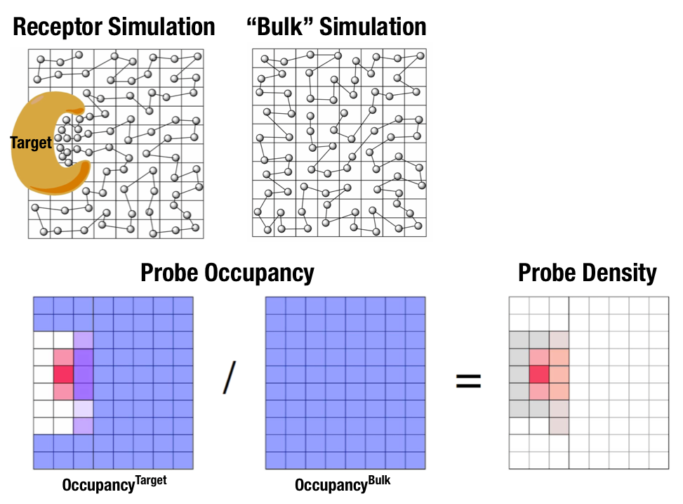
Fig. 1 Illustration of fragment density maps.

Fig. 1 illustrates FragMaps generation. Two MD simulations of a probe molecule (e.g., benzene) are performed in the presence of a protein and in aqueous solution (without protein), resulting in two occupancy maps, \(O^\mathrm{target}\) and \(O^\mathrm{bulk}\), respectively. The GFE (grid free energy) FragMaps are then derived by the following formula

\[\mathrm{GFE}^T_{x,y,z} = -RT \log \frac{O^\mathrm{target}_{x,y,z}}{\left< O^\mathrm{bulk} \right>}\]

By generating FragMaps using various small solutes representing different functional groups including benzene, propane, methanol, imidazole, formamide, acetaldehyde, methylammonium, acetate, and water, it is possible to map the functional group affinity pattern of a protein. FragMaps encompass the entire protein such that all FragMap types are in all regions. Thus, information on the affinity of all the different types of functional groups is available in and around the full 3D space of the protein or other target molecule.

FragMaps may be used in a qualitative fashion to facilitate ligand design by allowing the medicinal chemist to readily visualize regions where the ligand can be modified or functional groups added to improve affinity and specificity. As the FragMaps include protein flexibility, they indicate regions of the target protein that can “open” thereby identifying regions under the protein surface accessible for ligand binding. In addition to FragMaps, an “exclusion map” is generated based on regions of the system that are not sampled at all by water or probe molecules during the MD simulations. Therefore, the exclusion map represents a strictly inaccessible surface.

Many proteins contain binding sites that are partially or totally inaccessible to the surrounding solvent environment that may require partial unfolding of the protein for ligand binding to occur. SILCS sampling of such deep or inaccessible pockets is facilitated by the use of a Grand Canonical Monte Carlo (GCMC) sampling technique in conjunction with MD simulations [10]. Thus, the SILCS technology is especially well-suited for targeting the deep and inaccessible binding sites found in targets like GPCRs and nuclear receptors.

Once a set of ligand-independent SILCS FragMaps are produced, they can be used for various purposes that rapidly rank ligand binding in a highly computationally efficient manner for multiple ligands WITHOUT recalculating the FragMaps. Applications of SILCS methodology include:

• Binding site identification

  • Binding pocket searching with known ligands

  • Binding pocket identification via pharmacophore generation

  • Binding pocket identification via fragment screening

• Database screening

  • SILCS 3D pharmacophore models

  • Ligand posing using available techniques (Catalyst, etc)

  • Ligand ranking

• Fragment-based ligand design

  • Identification of fragment binding sites

  • Estimation of ligand affinity following fragment linking

  • Expansion of fragment types

• Ligand optimization

  • Qualitative ligand optimization by FragMaps visualization

  • Quantitative evaluation of ligand atom contributions to binding

  • Quantitative estimation of relative ligand affinities

  • Quantitative estimation of large numbers of ligand chemical transformations

SILCS generates 3D maps of interaction patterns of functional group with your target molecule, called FragMaps. This unique approach simultaneously uses multiple different small solutes with various functional groups in explicit solvent MD simulations that include target flexibility to yield 3D FragMaps that encompass the delicate balance of target-functional group interactions, target desolvation, functional group desolvation and target flexibility. The FragMaps may then be used to both qualitatively direct ligand design and quantitatively to rapidly evaluate the relative affinities of large numbers of ligands following the precomputation of the FragMaps.

This chapter goes over the workflow of generating and visualizing FragMaps.

Running SILCS simulations from the SilcsBio GUI

Please see SILCS simulation from the GUI as described in Graphical User Interface Quickstart for a step-by-step description for using the SilcsBio GUI for SILCS simulations.

FragMap generation using SILCS begins with a well-curated protein structure file (without ligand) in PDB file format. We recommend keeping only those protein chains that are necessary for the simulation, removing all unnecessary ligands, renaming non-standard residues, filling in missing atomic positions, and, if desired, modeling in missing loops. Please contact support@silcsbio.com if you need assistance with protein preparation.

A typical SILCS simulation can produce output totaling in excess of 100 GB, so please select a folder with appropriate free space.

The setup process automatically builds the topology of the simulation system, creating metal-protein bonds if metal ions are present, rotates side chain orientations to enhance sampling, and places probe molecules around the protein. The SilcsBio GUI provides Advanced Settings options prior to the setup process and prior to running the SILCS simulations.

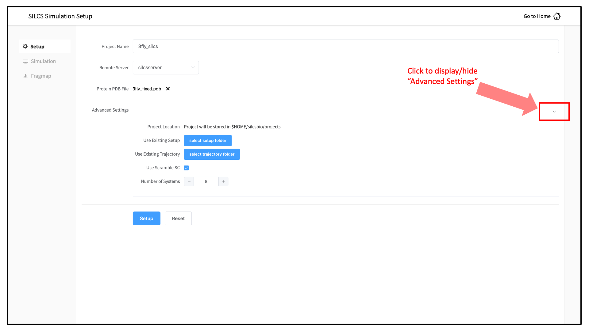
Tip

Default settings have been optimized for SILCS FragMap simulation. If you do wish to change the number of simulations to run or to run simulations with a different number of CPUs, you can make adjustments in the Advanced Settings options.

Tip

If a simulation stops prematurely, the progress bar will turn red and show a “Restart” option. When the job is restarted, the simulation will continue from the last cycle, but the progress bar may reset. This is because job recovery iterates over existing cycles to check if output was correctly produced. The completed cycles will be automatically skipped and the progress will update to where the job had stopped. That is to say, restarting a failed or stopped job will not cause you to lose existing job progress.

Running SILCS simulations from the command line interface

Please see SILCS simulation from the command line as described in Command Line Interface Quickstart for a step-by-step description for using the Command Line Interface (CLI) for SILCS simulations.

FragMap generation using SILCS begins with a well-curated protein structure file (without ligand) in PDB file format. We recommend keeping only those protein chains that are necessary for the simulation, removing all unnecessary ligands, renaming non-standard residues, filling in missing atomic positions, and, if desired, modeling in missing loops. Please contact support@silcsbio.com if you need assistance with protein preparation.

SILCS simulation setup

${SILCSBIODIR}/silcs/1_setup_silcs_boxes prot=<Protein PDB>

Warning

The setup program internally uses the GROMACS utility pdb2gmx, which may have problems processing the protein PDB file. The most common reasons for errors at this stage involve mismatches between the expected residue name/atom names in the input PDB and those defined in the CHARMM force-field.

To fix this problem: Run the pdb2gmx command manually from within the 1_setup directory for a detailed error message. The setup script already prints out the exact commands you need to run to see this message.

cd 1_setup
pdb2gmx –f <PROT PDB NAME>_4pdb2gmx.pdb –ff charmm36 –water tip3p –o test.pdb –p test.top -ter -merge all

Once all the errors in the input PDB are corrected, rerun the setup script.

The setup command offers a number of options. The full list of options can be reviewed by simply entering the command without any options:

$SILCSBIODIR/silcs/1_setup_silcs_boxes
This script will setup Topology/PDB for SILCS simulations

Usage: $SILCSBIODIR/silcs/1_setup_silcs_boxes prot=<protein PDB file>

Optional Parameters:
   numsys=<# of simulations; default=10>
   skip_pdb2gmx=<true/false; default=false>
   lig=<lig.mol2; default=empty/NULL>
   core_restraint_string=<restrained residues, e.g., "r 17-21 | r 168-174"; default=all>
   scramblesc=<true/false; default=true>
   margin=<system margin in Angstrom; default=15>
   halogen=<true/false; default=false>

• core_restraint_string: By default, a weak harmonic positional restraint, with a force constant of ~0.1 kcal/mol/Ų, is applied to all C-alpha atoms during SILCS simulations. This option lets you modify this default.

  For example, if core_restraint_string="r 17-160 | r 168-174" is supplied, then only the C-alpha atoms in residues 17 to 160 and residues 168 to 174 will be restrained.

SILCS GCMC/MD simulation

Following completion of the setup, run 10 GCMC/MD jobs using the following script:

${SILCSBIODIR}/silcs/2a_run_gcmd prot=<Protein PDB>

This script will submit 10 jobs to the predefined queue. Each job runs out 100 ns of GCMC/MD with the protein and the solute molecules.

Once the simulations are complete, the 2a_run_gcmd/[1-10] directories will contain *.prod.125.rec.xtc trajectory files. If these files are not generated, then your simulations are either still running or stopped due to a problem. Look in the log files within these directories to diagnose problems.

FragMap generation

Once your simulations are done, generate the FragMaps using the following command:

${SILCSBIODIR}/silcs/2b_gen_maps prot=<Protein PDB>

This will submit 10 single-core jobs that will build occupancy maps (FragMaps) spanning the simulation box for select probe molecule atoms representing different functional groups. For a ~50K atom simulation system, this step takes approximately 10-20 minutes to complete. The FragMaps have a default grid spacing of 1 Å.

The next step is to combine the occupancy FragMaps generated from individual simulations and convert them into GFE FragMaps. Each voxel in a GFE FragMap contains a Grid Free Energy (GFE) value for the probe type that was used to create the corresponding occupancy FragMap.

${SILCSBIODIR}/silcs/2c_fragmap prot=<Protein PDB>

GFE FragMaps will be created in the silcs_fragmap_<protein PDB>/maps directory. PyMOL and VMD scripts to load these file will be created in the silcs_fragmap_<protein PDB> directory.

<prot name>.benc.gfe.map    Aromatic map
<prot name>.prpc.gfe.map    Aliphatic map
<prot name>.aceo.gfe.map    Charged acceptor map
<prot name>.mamn.gfe.map    Charged donor map
<prot name>.forn.gfe.map    Polar nitrogen donor map (Formamide)
<prot name>.foro.gfe.map    Polar oxygen acceptor map (Formamide)
<prot name>.imin.gfe.map    Polar nitrogen acceptor map (Imidazole)
<prot name>.iminh.gfe.map   Polar nitrogen donor map (Imidazole)
<prot name>.aalo.gfe.map    Polar oxygen acceptor map (Acetaldehyde)
<prot name>.meoo.gfe.map    Polar oxygen acceptor map (Methanol)
<prot name>.apolar.gfe.map  Generic Apolar maps
<prot name>.hbdon.gfe.map   Generic donor maps
<prot name>.hbacc.gfe.map   Generic acceptor maps
<prot name>.excl.map        Exclusion map
<prot name>.ncla.map        Zero map

Cleanup

Raw trajectory files are large. To reduce file sizes, hydrogen atom positions can be deleted with the following:

${SILCSBIODIR}/silcs/2d_cleanup prot=<Protein PDB>

SILCS simulation setup with GPCR targets

You may use either a bare protein structure or your own pre-built protein/bilayer system with SILCS.

If you are beginning with a bare protein, SilcsBio provides a command line utility to embed transmembrane proteins, such as GPCRs, in a bilayer of 9:1 POPC/cholesterol for subsequent SILCS simulations:

${SILCSBIODIR}/silcs-memb/1a_fit_protein_in_bilayer prot=<Protein PDB>

This command will align the first principal axis of the protein with the bilayer normal (Z-axis) and translate the protein center of the mass to the center of the bilayer (Z=0).

If the protein is already oriented as desired, orient_principal_axis=false will suppress automatic principal axis-based alignment.

${SILCSBIODIR}/silcs-memb/1a_fit_protein_in_bilayer prot=<Protein PDB> orient_principal_axis=false

By default the system size is set to 120 Å along the X and Y dimensions. To change the system size, use the bilayer_x_size and bilayer_y_size options.

${SILCSBIODIR}/silcs-memb/1a_fit_protein_in_bilayer prot=<Protein PDB> bilayer_x_size=<X dimension> bilayer_y_size=<Y dimension>

The resulting protein/bilayer system will be output in a PDB file with suffix _popc_chol. It is important to use molecular visualization software at this stage to confirm correct orientation of the protein and size of the bilayer before using this output as the input in the next step.

Alternatively, you may use a protein/bilayer system that has been built using other software tools.

The following command will prepare the SILCS simulation box by adding water and probe molecules to the protein/bilayer system:

${SILCSBIODIR}/silcs-memb/1b_setup_silcs_with_prot_bilayer prot=<Protein/bilayer PDB>

SILCS GCMC/MD simulation can now be launched with the following command:

${SILCSBIODIR}/silcs/2a_run_gcmd prot=<Protein/bilayer PDB> memb=true

The SILCS GCMC/MD will begin with a 6-step pre-equilibration to slowly relax the bilayer followed by 10 ns of relaxation of the protein into the bilayer prior to the production simulation.

Tip

GPCR simulation systems are typically large and can require significant storage space (> 200 GB) and simulation time (> 14 days with GPUs).

FragMap generation from the GCMC/MD simulation data follows the same protocol as for non-bilayer systems. Refer to previous instructions for $SILCSBIODIR/silcs/2b_gen_maps and $SILCSBIODIR/silcs/2c_fragmap.

If you encounter a problem, please contact support@silcsbio.com.

SILCS simulation setup with halogen probes

SILCS probes with halogen-containing functional groups can be useful for extending the diversity of chemical space covered by FragMaps. While a common approach is to consider halogen atoms as non-polar groups, research on non-covalent “halogen bonding” suggests halogen atoms warrant special treatment.

The CHARMM General Force Field CGenFF v.2.3.0+ allows halogen atoms to be treated with lonepairs to achieve directionality in polar interactions. These force field improvements are included in SILCS simulations from version 2020.1 of the SilcsBio software, and halogen-protein interactions can be determined using a set of halogenated probes in SILCS simulations.

To include halogenated probes in your simulation, add the halogen=true keyword:

${SILCSBIODIR}/silcs/1_setup_silcs_boxes prot=<Protein PDB> halogen=true
${SILCSBIODIR}/silcs/2a_run_gcmd prot=<Protein PDB> halogen=true
${SILCSBIODIR}/silcs/2b_gen_maps prot=<Protein PDB> halogen=true
${SILCSBIODIR}/silcs/2c_fragmaps prot=<Protein PDB> halogen=true

This will create folders ending with _x (i.e., 1_setup_x/, etc.) to denote SILCS-Halogen simulation systems, as opposed to standard SILCS simulations. While the SilcsBio GUI does not currently support running such jobs, it will automatically load FragMaps from these simulations alongside standard FragMaps.

If you encounter a problem, please contact support@silcsbio.com.

Resuming stopped SILCS jobs

Situations such as exceeding workload manager (job queue) walltime limits can cause SILCS jobs to stop before running to completion. Resuming such jobs from where they stopped is straightforward. On the server where the job was running, go to the directory <Project Location>/2a_run_gcmd/i, where i is an integer from 1 to 10 and corresponds to the stopped job among the ten SILCS GCMC/MD jobs that were being run for that particular target. In that directory, directly use the file job_mc_md.cmd to submit the job to the workload manager, for example qsub job_mc_md.cmd for Sun Grid Engine (SGE) and sbatch job_mc_md.cmd for Slurm.

To ensure a successful restart, make sure to issue any required extra setup commands (for example, as listed in the “Extra setup” field under Settings and remote server configuration from the SilcsBio GUI Home screen) such as export LD_LIBRARY_PATH=<path/to/cuda/libraries> or module load <name of cuda module> before submitting the job.

Visualizing FragMaps with external software (MOE, PyMol, VMD)

Whether you used the SilcsBIO GUI or the 2c_fragmap command line utility to create SILCS FragMaps from your SILCS simulation trajectories, you will have a folder silcs_fragmap_<protein PDB>/maps that contains SILCS grid free energy (GFE) FragMaps for you system. SILCS FragMaps are defined using non-hydrogen atoms, and for certain solute types (imidazole, formamide) there are multiple FragMaps. FragMaps for water oxygen atoms (tipo) are created to identify water molecules that can be difficult to displace. Generic FragMaps for apolar (benzene+propane), H-bond donor (neutral H-bond donors), and H-bond acceptor (neutral H-bond acceptors) probe types are included to simplify visual analysis.

The easiest way to visualize FragMaps is with the SilcsBio GUI. SilcsBio also provides convenient FragMap visualization using MOE, PyMOL, and VMD.

FragMaps in MOE

To visualize your SILCS FragMaps with MOE, first create FragMaps in the MOE-readable CNS format. For this example, if your jobs ran on your server in the directory ~/silcsbio/projects/silcs.5tGP:

cd ~/silcsbio/projects/silcs.5tGP
$SILCSBIODIR/silcs/2c_fragmap prot=<Protein PDB> cns=true

Note

This step is required ONLY for visualization with MOE. CNS format grid files are approximately 10x the size of the default-format grid files generated and used by your SilcsBio software. PyMol and VMD are capable of reading the default-format files, and, to save disk space, CNS format files are not generated unless specifically specified using the above command.

Running this command will create CNS format FragMap files in the silcs_fragmap_<protein PDB>/maps directory. It will also create the file silcs_fragmap_<protein PDB>/view_maps.svl. First, copy the entire silcs_fragmap_<protein PDB> directory from your server to a convenient location on the desktop or laptop machine where you will be doing the visualization. For example, on Linux or MacOS, you may use a command like

scp -rp silcsbio@silcsserver:~/silcsbio/projects/silcs.5tGP/silcs_fragmaps_3fly_fixed ~/Desktop

Then, use MOE to open the silcs_fragmap_<protein PDB>/view_maps.svl file by selecting File ‣ Open, which will bring up the “Open” window. In this window, browse to the silcs_fragmap_<protein PDB> directory, which, in this example, was downloaded from the server to the Desktop of the machine on which we are doing the visualization. Click the “CWD” button in the upper right corner to set this directory as the “Working Folder.” Then, select the view_maps.svl file and click the “Open” button:

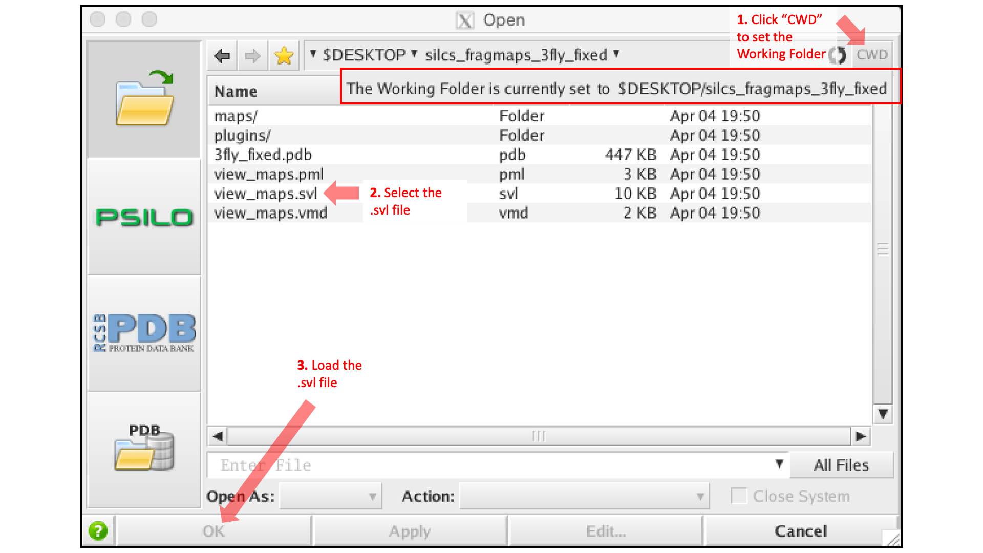
MOE will process the view_maps.svl file to load your input PDB structure <protein PDB>.pdb used for the SILCS simulations, the CNS format FragMap files <protein PDB>.<fragmaptype>.map.cns, and the Exclusion Map <protein PDB>.excl.map.cns. The visualization of the FragMaps and Exclusion Map can be controlled in the “Surfaces and Maps” window, which is also automatically loaded by view_maps.svl.

FragMaps in PyMol

First, copy the entire silcs_fragmap_<protein PDB> directory from your server to a convenient location on the desktop or laptop machine where you will be doing the visualization. For example, on Linux or MacOS, you may use a command like

scp -rp silcsbio@silcsserver:~/silcsbio/projects/silcs.5tGP/silcs_fragmaps_3fly_fixed ~/Desktop

If your operating system associates the .pml extension with PyMol, simply double click on the view_maps.pml file in the silcs_fragmaps_<protein PDB> folder. Otherwise, open PyMol, select File ‣ Open…, and open the view_maps.pml file. It is also possible to do this by typing commands into the PyMol console. For the silcs_fragmaps_3fly_fixed example here, the commands would be

cd /Users/silcsbio/Desktop/silcs_fragmaps_3fly_fixed

which sets the working directory, and

run view_maps.pml

which runs the view_maps.pml file in that directory.

Whichever of these three methods you use to load view_maps.pml, PyMol wil load the PDB structure <protein PDB>.pdb used for the SILCS simulations, the FragMap files, and the Exclusion Map. The visualization of the FragMaps and Exclusion Map can be controlled in the “PyMol FragMap Tools” window, which is also automatically loaded by view_maps.pml.

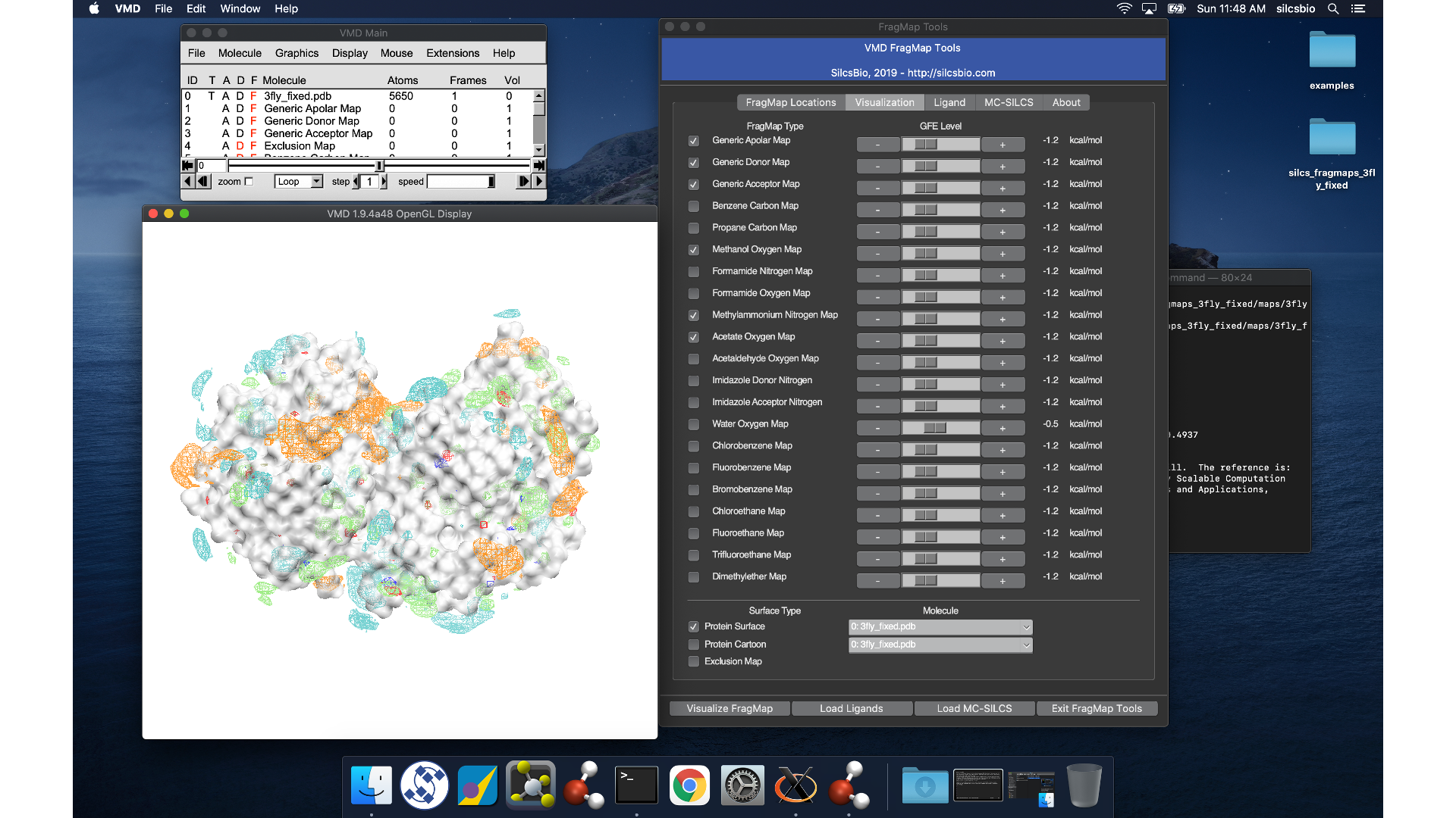
FragMaps in VMD

First, copy the entire silcs_fragmap_<protein PDB> directory from your server to a convenient location on the desktop or laptop machine where you will be doing the visualization. For example, on Linux or MacOS, you may use a command like

scp -rp silcsbio@silcsserver:~/silcsbio/projects/silcs.5tGP/silcs_fragmaps_3fly_fixed ~/Desktop

Open VMD, select File ‣ Load Visualization State…, and open the view_maps.vmd file located in the silcs_fragmap_<protein PDB> directory you downloaded. A new window will pop up that says, “Select the folder where silcs_fragmap folder is downloaded”. Click the “OK” button and select the silcs_fragmap_<protein PDB> you downloaded.

Tip

Be careful to select the silcs_fragmap_<protein PDB> folder and NOT the silcs_fragmap_<protein PDB>/maps folder.

VMD wil load the PDB structure <protein PDB>.pdb used for the SILCS simulations, the FragMap files, and the Exclusion Map. The visualization of the FragMaps and Exclusion Map can be controlled in the “VMD FragMap Tools” window, which is also automatically loaded by view_maps.vmd.