SILCS-Pharm

Background

Three-dimensional (3D) pharmacophore models (also called “hypotheses”) offer an intuitive and powerful approach for virtual screening (VS). 3D pharmacophore VS works by searching for matches between the 3D pattern of functional groups constituting a pharmacophore model and the 3D arrangement of functional groups in ligand conformers in a virtual database. Ligands having conformers that closely match the pharmacophore model are considered hits. Traditionally, 3D pharmacophore models were developed using experimental knowledge of the binding poses for ligands to a receptor. This is in contrast to energy function-based VS (“docking”). An advantage of docking approaches was that they only require experimental knowledge of the receptor structure, and not of bound ligands. However, it is possible to develop pharmacophore models using only the receptor structure. One means to generate such receptor-based pharmacophore models is with data from SILCS simulations.

SILCS-Pharm converts Grid Free Energy (GFE) FragMaps into 3D pharmacorphore models. GFE FragMaps from SILCS simulations are used as inputs for the four-step SILCS-Pharm process:

voxel selection;
voxel clustering and FragMap feature generation;
FragMap feature to pharmacophore feature conversion;
generation of a pharmacophore model for virtual screening (VS).

Here, “feature” refers to the identity and location of a chemical functional group and “pharmacophore model” is a collection of pharmacophore features.

FragMap generation from SILCS MD entails partitioning 3D space into uniform cubic voxels and enumerating fragment binding probabilities for each voxel. The voxels are retained during Boltzmann-inversion of probabilities to create GFE FragMaps. As the GFE voxel value represents the binding strength of a functional group at that specific location on the protein surface, the first step identifies the most favorable interactions based on a particular GFE cutoff value. In the second step, clustering is performed to group adjacent voxels, with each unique cluster becoming a FragMap feature. In the third step, the FragMap features are classified and converted into pharmacophore features. Finally, the pharmacophore features are prioritized using Feature GFE (FGFE) scores to create a SILCS 3D pharmacophore model [13]. In the current scheme, the program searches through five FragMap types: Generic Apolar, Generic Donor, Generic Acceptor, Positively Charged, and Negatively Charged. Additionally, instead of using a rigidly-defined protein surface to determine regions that ligands cannot sample because of protein volume occlusion, the SILCS Exclusion Map is used. The Exclusion Map has been validated to be a better alternative to more traditional representations of the occluded volume of the protein, and it explicitly accounts for protein flexibility.

Running SILCS-Pharm

SILCS-Pharm Using the SilcsBio GUI

Begin a new SILCS-Pharm project:

Select New SILCS-Pharm project from the Home page.
Enter a project name and input files:

Enter a project name. Then, provide FragMap and protein input files. You may choose these files from the computer where you are running the SilcsBio GUI (“localhost”) or from any server you have previously configured, as described in File and Directory Selection. Once all information is entered correctly, press the “Setup” button at the bottom of the page.
Define the ligand binding pocket:

After pressing the “Setup” button at the bottom of the page, the screen will update to add “Pharmacophore Search” to the list of information. Click the “Select Pocket” button on the right-hand side of the window.

The GUI will now be showing the protein molecular graphic in the center pane. On the right-hand side, in the “Pocket” tab, you will need to define the pocket center based on the center-of-geometry of a ligand pose (“Define Pocket using Ligand”), or a target residue selection (“Define Pocket using Selection”), or by directly entering an x, y, z coordinate (“Define Pocket by XYZ”). You will also need to choose a radius (default value “10”) to complete the definition of the spherical pocket. If it is difficult to see the spherical pocket definition in the center pane, hide the protein surface representation. Click on the “Save Pocket” button and the “OK” acknowledgement to continue.
Run SILCS-Pharm:

You will be returned to the previous screen, which now includes “Sampling Region” information consisting of the spherical pocket center and radius. You will also see default FragMap cutoff values listed for selection of FragMap densities for creation of pharmacophore features. You may adjust those values if you desire. Click on the “Run SILCS-Pharm” button to run the four-step SILCS-Pharm process.

A pop-over window will appear and show job output, and the job will run to completion in a matter of seconds. Click the green “Search Finished” button.
Visualize and save pharmacophore models:

After clicking the green “Search Finished” button, the GUI will allow you to visualize the pharmacophore features on the protein. You may wish to click on the “Protein” tab in the right-hand panel and deselect the protein for a cleaner view of the pharmacophore features in the field of fragmaps.

The “Pharmacophore” tab will list all the pharmacophore features automatically generated from the FragMaps. You may adjust the radii of the individual features or deselect them entirely. You can also determine the distance between any two features to assist your analysis and choices.

Once finished with pharmacophore feature selection and adjustment, click the “Save Feature” button. You have the option to save the features in either Pharmer or MOE formats. This will allow you to save your pharmacophore model containing your selected/adjusted features in .ph4 format on your local computer. By selecting/adjusting different subsets of the pharmacophore features, including the Exclusion Map, you may create multiple different pharmacophore models and save each one as a separate .ph4 file. Note that exclusion pharmacophore features are NOT supported by Pharmer. This capability allows for different pharmacophore model screens of a binding site. The resulting diverse hits from those screens can be combined and, for example, subjected to SILCS-MC Pose Refinement for rescoring. Pre-existing pharmacophore models saved in .ph4 format can also be viewed and edited through View/Edit Pharmacophore File on the “Home” page (see View and Edit Pharmacophore Files for more details).

SILCS-Pharm Using the CLI

A single command line interface command performs the four-step SILCS-Pharm process:

${SILCSBIODIR}/silcs-pharm/1_calc_silcs_pharm prot=<prot pdb> center="x,y,z"

The input arguments are the PDB file used for the SILCS run and the absolute position of the center of a 10 Å sphere to be used to define the boundaries of the pharmacophore model. Two output files result from this command. <prot>.keyf_<#features>.ph4 can be directly used for 3D pharmacophore VS by compatible programs (see below for generating Pharmer-compatible ph4 files). <prot>_silcspharm_features.pdb provides output in PDB format for easy visualization using standard molecular graphics packages. Running the command with no arguments

${SILCSBIODIR}/silcs-pharm/1_calc_silcs_pharm

will list additional options. Along with the required arguments of prot=<prot pdb> and center="x,y,z", the following additional options can be set.

Optional parameters:

FragMap directory path:
mapsdir=<location and name of directory containing FragMaps; default=maps>
By default, the program will search for FragMaps in the maps directory.
Output directory path:
outputdir=<location and name of output directory; default=5_pharm>
By default, the program creates the directory 5_pharm and places all output files there.
Radius:
radius=<default: 10>
By default, a radius of 10 Å centered at center="x,y,z" is searched to generate pharmacophore features from the input FragMaps.
Generic Apolar FragMap cutoff:
apolar_cutoff=<default: -1.2>
By default, Generic Apolar FragMap voxels having a GFE value <= -1.2 kcal/mol are selected.
Generic Donor FragMap cutoff:
hbdon_cutoff=<default: -1.0>
By default, Generic Donor FragMap voxels having a GFE value <= -1.0 kcal/mol are selected.
Generic Acceptor FragMap cutoff:
hbacc_cutoff=<default: -1.0>
By default, Generic Acceptor FragMap voxels having a GFE value <= -1.0 kcal/mol are selected.
Methylammonium N FragMap cutoff:
mamn_cutoff=<default: -1.8>
By default, Methylammonium N FragMap FragMap voxels having a GFE value <= -1.8 kcal/mol are selected.
Acetate O FragMap cutoff :
aceo_cutoff=<default: -1.8>
By default, Acetate O FragMap FragMap voxels having a GFE value <= -1.8 kcal/mol are selected.

In addition to visualization, the output PDB file <prot>_silcspharm_features.pdb can be used for easy editing of the pharmacophore model. Using a text editor, modify/reduce the features in this file as desired and save the revised file as <prot>_silcspharm_features_revised.pdb. Using this revised PDB file and the original ph4 file <prot>.keyf_<#features>.ph4 as input, create a new ph4 file with:

${SILCSBIODIR}/programs/revise_ph4 <prot>.keyf_<#features>.ph4 <prot>_silcspharm_features_revised.pdb

The output of this command will be the revised ph4 file <prot>.keyf_<#features>_revised.ph4. To create Pharmer-compatible ph4 output, add the pharmer option:

${SILCSBIODIR}/programs/revise_ph4 <prot>.keyf_<#features>.ph4 <prot>_silcspharm_features_revised.pdb pharmer

Example Case Using the CLI

The following example demonstrates use of SILCS-Pharm from the command line interface to generate a pharmacophore model for p38 MAP kinase. Input files, including FragMaps, are provided in ${SILCSBIODIR}/examples/silcs/ (these same input files may also be used for a trial run of SILCS-Pharm with the SilcsBio GUI).

The x,y,z coordinates of the center of the complexed ligand are used to create a SILCS-Pharm 3D pharmacophore model encompassing the ligand binding site (shown below). These coordinates define the center of the sphere within which FragMap voxels are searched and clustered to generate features.

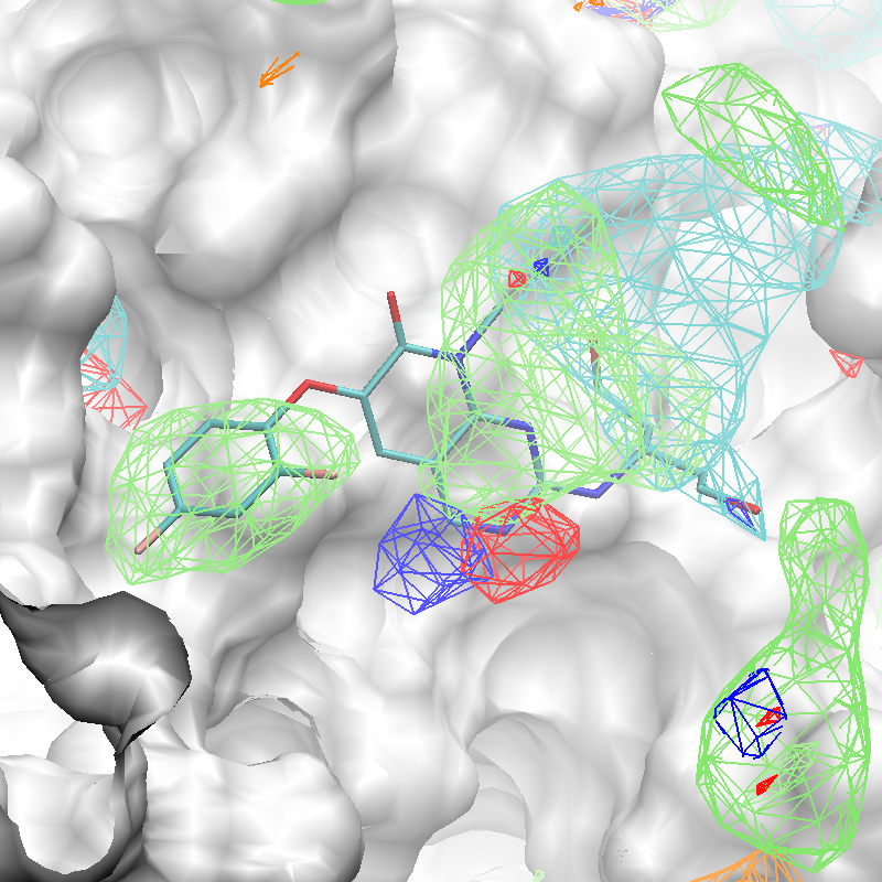
Using the ligand center coordinates center="35.24, 27.48, 37.73", generate the 3D pharmacophore model with:

${SILCSBIODIR}/silcs-pharm/1_calc_silcs_pharm prot=3fly.pdb center="35.24,27.48,37.73" mapsdir=${SILCSBIODIR}/examples/silcs/silcs_fragmaps_3fly/maps

The command will complete after several seconds, and the output will note, “A total of 13 features have been detected.” All output files will be in a new subdirectory 5_pharm. Standard molecular graphics software can be used to visualize the output file 3fly_silcspharm_features.pdb, which has one ATOM entry for each of the 13 pharmacophore features:

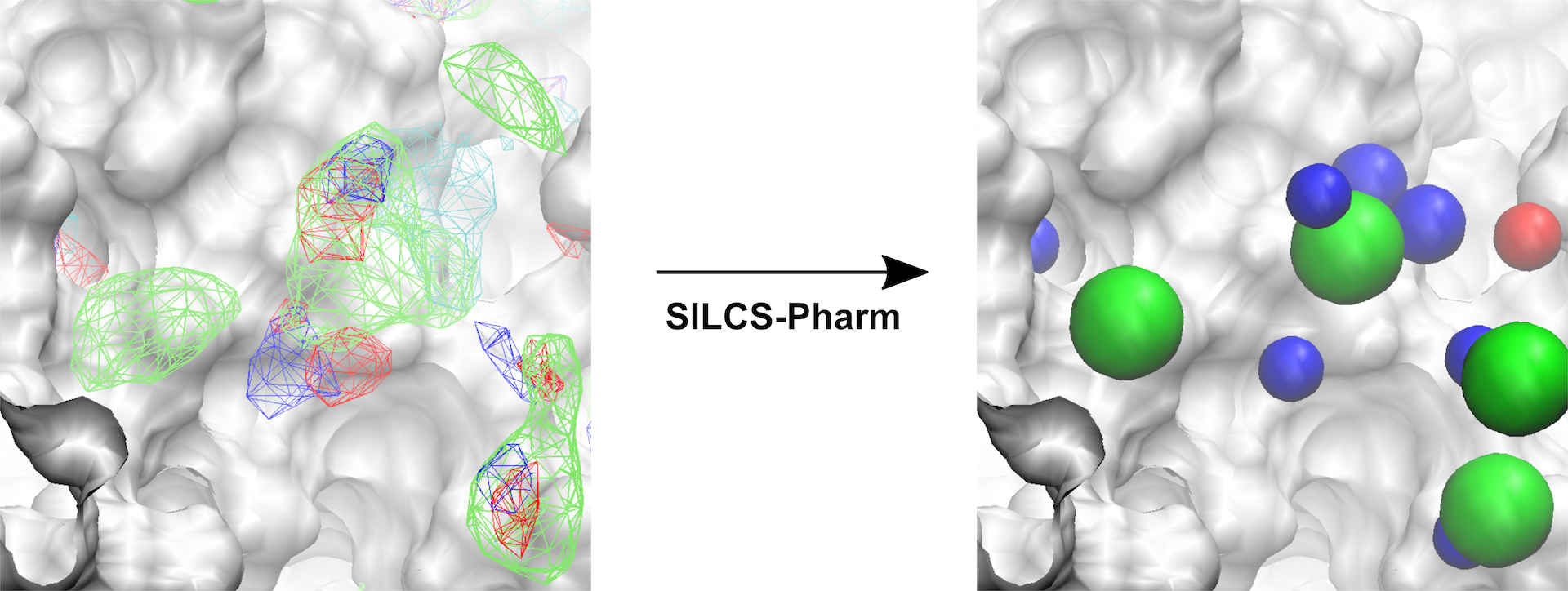
The conversion of FragMaps (left) to SILCS pharmacophore features (right) is shown above.

To modify/reduce the features, edit the output file 3fly_silcspharm_features.pdb and save it as 3fly_silcspharm_features_revised.pdb, then run ${SILCSBIODIR}/programs/revise_ph4:

${SILCSBIODIR}/programs/revise_ph4 3fly.keyf_13.ph4 3fly_silcspharm_features_revised.pdb

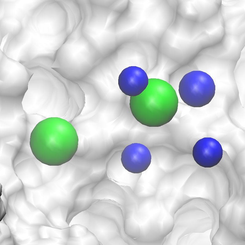
The output 3fly.keyf_13_revised.ph4 will reflect your revisions in 3fly_silcspharm_features_revised.pdb. Below are the revised SILCS pharmacophore features.

Pharmacophore Screening with Pharmer

Through the integration of Pharmer, an open-source pharmacophore search program, into the SilcsBio software, users are able to perform high-throughput virtual screening (HTVS) using pharmacophore features generated by SILCS-Pharm. To perform HTVS with Pharmer, please follow the steps detailed in this section.

Check Pharmer installation:

Make sure that your Pharmer program is installed correctly using the following command:

$SILCSBIODIR/programs/pharmer --help

If the above command produces an error, please see PHARMER Installation.

Check database imports:

High-throughput virtual screening (HTVS) requires a prepared database of screening compounds. SilcsBio users can get Ready-To-Screen Pharmer compatible databases that include multiple protomers and conformers of each screening compound upon request. Please contact support@silcsbio.com to request a prepared database. Alternatively, users may also choose to build their databases locally. Instructions on how to build a database are provided in Building a Pharmer-Compatible Database.

Once the database has been prepared, ensure that the database is linked to SILCSBIODIR using the following command:

ls $SILCSBIODIR/data/databases/pharmer_databases

The above command will output a list of available databases.

If the above command results in an empty output or the desired database is not listed, then please follow the steps below to link a database (e.g., molport) to SILCSBIODIR.

# create the directory for your database
mkdir -p $SILCSBIODIR/data/databases/pharmer_databases/molport

# create symbolic links for parts of your prepared database
ln -s Part_* $SILCSBIODIR/data/databases/pharmer_databases/molport/

Run Pharmer to perform virtual screening:

With both Pharmer installed and the appropriate database(s) linked, users can perform HTVS on a pharmacophore model using the command below:

$SILCSBIODIR/silcs-pharm/2_run_pharmer ph4=<PH4 file> database=<database to screen>

Required parameters:

Path and name of the input pharmacophore model in .ph4 format:
ph4=<PH4 file>
The .ph4 file containing your pharmacophore model must be in Pharmer format. If you do not have a .ph4 file, please refer to Running SILCS-Pharm to create one.
Name of the database to screen:
database=<database to screen>
You may include multiple databases in your virtual screening project by providing space-separated names (e.g., database="molport enamine").

Optional parameters:

Name of the directory containing the output:

outputdir=<location and name of output directory; default=5_pharm>

Path to the Pharmer program executable:

pharmer=<location and name of Pharmer executable; default=$SILCSBIODIR/programs/pharmer>

Number of processors available for running the Pharmer program:
nproc=<# of cores available to Pharmer; default nproc=8>
The default number of processors used is determined when the SilcsBio Software is set up on the server on which the calculations are performed.

Warning

The Pharmer program does not support pharmacophore features representing the Exclusion Map.

Note

It is imperative that the selected database(s) is a conformational database, which includes a representative set of conformers for each molecule. Pharmer screening entails only rigid translations and rotations of the entire molecule; NO internal rotations of torsion angles are performed. For assistance in creating a custom conformer database, please contact us at support@silcsbio.com.

Building a Pharmer-Compatible Database

Pharmer requires a database of molecules to screen. The database should be in Pharmer format, which includes multiple protomers and conformers of each screening compound. The database should also be in a directory structure that is accessible to the computer on which 2_run_pharmer command (step 3 under Pharmacophore Screening with Pharmer) will be run.

To build a Pharmer-compatible database, follow the steps below:

1. Collect structures of all molecules of interest in one SDF file: Prepare an SDF file containing all of the molecules you want to screen. Make sure to enumerate protomers for each molecule. Alternately, those with access to CCG’s MOE will have the option to use MOE (sdwash) to wash and enumerate protomers.

Tip

Note that the SDF file may contain a property with unique identifier for each molecule. The property name can be used to rename the molecules in the database.

Build the Pharmer-compatible database:

After preparing the SDF file containing all molecules of interest, run the build_pharmer_database command:

$SILCSBIODIR/silcs-pharm/build_pharmer_database dbname=<database name> sdfile=<location and name of SDF file of the compounds>

Required parameters:

Name of the output database (e.g. molport_2024_01):
dbname=<database name>
Please use alphanumeric characters, dashes, and underscores only. The database name will be used to create the directory structure for the database.
Path and name of SDF file of the compounds:
sdfile=<location and name of SDF file of the compounds>
This is the SDF file containing the molecules to be screened. The SDF file can have 2D or 3D coordinates. No hydrogen atoms are required in the SDF file as they will be added by RDKit.

Optional parameters:

Number of conformers to generate:
nconformers=<# of conformers to generate; default=10>
The default number of conformers to generate is 10. An RMSD threshold of 0.35 Å is used to filter out similar conformers.
Number of molecules per part:
molsperpart=<# of molecules per part; default=50000>
The output database will be divided into parts, with each part containing a specified number of molecules. The default number of molecules per part is 50,000. The number of parts will be determined by the number of molecules in the database. The parts will be named Part_1, Part_2, etc.
The number of the first part:
firstpart=<first part number; default=1>
The default number of the first part is 1. This option is used to specify the number of the first part in the database. This may be useful if you are appending new parts to an existing database. This may also be useful if you are building a large database requiring the use of different storage locations for additional parts.
Unique identifier property in SDF file:
molid=<unique identifier property in SDF file to set molecule name>
The value of this property will be used to rename the molecules in the database during the washing stage. Combined with the prefix parameter, users can use this option to rename the molecules in the database as <prefix>_<molid>. For example, molid="PUBCHEM_EXT_DATASOURCE_REGID" is a unique identifier property for the SDF files of the MolPort database.
Prefix for the molecule names:
prefix=<a prefix for the molecule name>
The specified prefix will be added to the molecule name in the database. If you used the molid parameter, the molecule name will be the value of the property in the SDF file with the prefix added.
Skip the washing and enumeration of protomers:
skipwash=<skip washing and protomer generation; true/false; default=false>
If you have already washed and enumerated protomers for the molecules in the SDF file, you can skip this step by setting skipwash=true. This option can NOT be used with the moewash option. Also, this option should NOT be used if you want to use molid and prefix options.

Number of cores available to Pharmer:

nproc=<# of cores available to Pharmer; default=8>

Path to the Python executable for RDKit:

python=<path to python executable for rdkit; default=$(which python)>

Add newly created database to default path:
addtopath=<move the database to pharmer_databases directory; true/false; default=false>
Use this option if you want to make the database available in the default dbpath for pharmacophore screening with the 2_run_pharmer script. Setting this option to true will copy the database to the $SILCSBIODIR/data/databases/pharmer_databases directory. Alternative options are:
1. Create a symbolic link of the database directory in the default dbpath (i.e., $SILCSBIODIR/data/databases/pharmer_databases) directory. Note that the original database should be accessible from the compute node where the screening job scripts (job_pharmer*cmd) get submitted. Individual parts of the database could also be linked separately if certain parts are stored in different locations. It is okay if the symbolic links are inactive on the login node.
2. Use the dbpath option in the 2_run_pharmer script to specify the location of the database. Again, the database should be accessible from the compute node where the screening job scripts (job_pharmer*cmd) get submitted.

Additional parameters:

Use MOE by CCG to wash and enumerate protomers:

moewash=<use MOE to wash and enumerate protomers; true/false; default=false>

Path to the MOE (sdwash) executable for washing:

sdwash=<path to MOE(sdwash) executable for washing; default=>

Number of protomers to generate:

nprotomers=<# of protomers to generate; default=3>

Number of MOE tokens available to use:

moetokens=<number of MOE tokens available; default=3>