Graphical User Interface Quickstart

This chapter provides a step-by-step introduction on how to use the SilcsBio Graphical User Interface (GUI).

Remote server setup

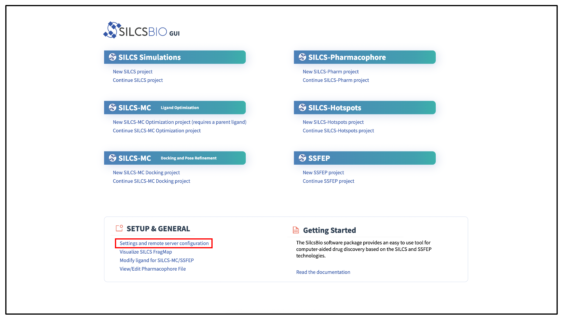
The SilcsBio GUI is designed to work with the server installation of the SilcsBio software. When you launch the GUI, you will be presented with the Home page. From the Home page, select Settings and remote server configuration.

Within the “Settings” page, select Server and enter the remote server information, such as Server Address (IP address), Username, and an SSH key to the server. If you do not have an SSH key to the server, leave it blank. The GUI will ask you the password to the remote server instead. Select the “Make Default Server” checkbox if you would like to set this server as your default server. This server will be selected as a default in other parts of the GUI.

You will also need to enter SILCSBIODIR and GMXDIR file path values. These should match the values on your server. You may use the “Extra setup” field to pass additional commands to the server, such as exporting environment variables or loading modulefiles. You may use the “Project Directory” field to define the directory on your server where server job input files will be created and server job outputs stored. Typical SILCS simulations produce output files in excess of 100 GB, so please select a project directory file folder with appropriate storage capacity. The “SILCS NUMSYS” field determines how many SILCS jobs are launched for creating FragMaps. Set this to an even integer; we recommend “10” to maximize convergence or “8” to minimize resource use.

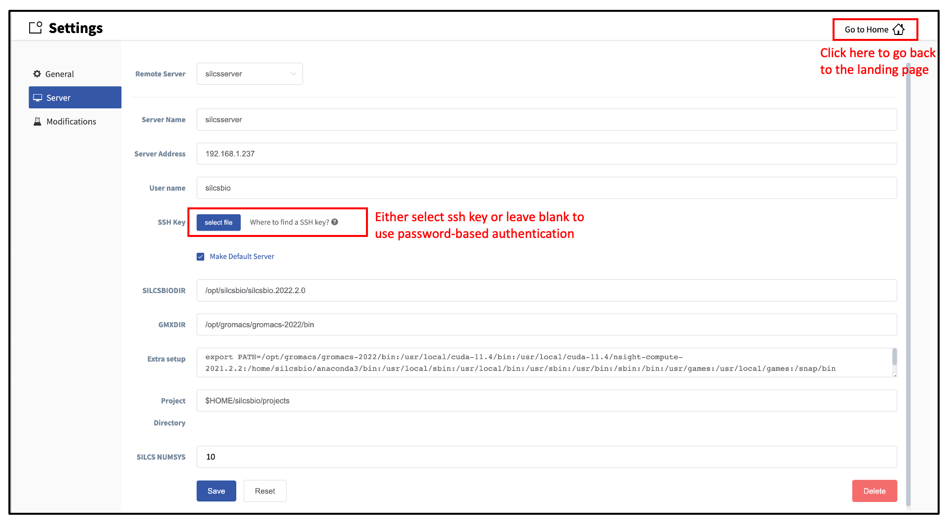
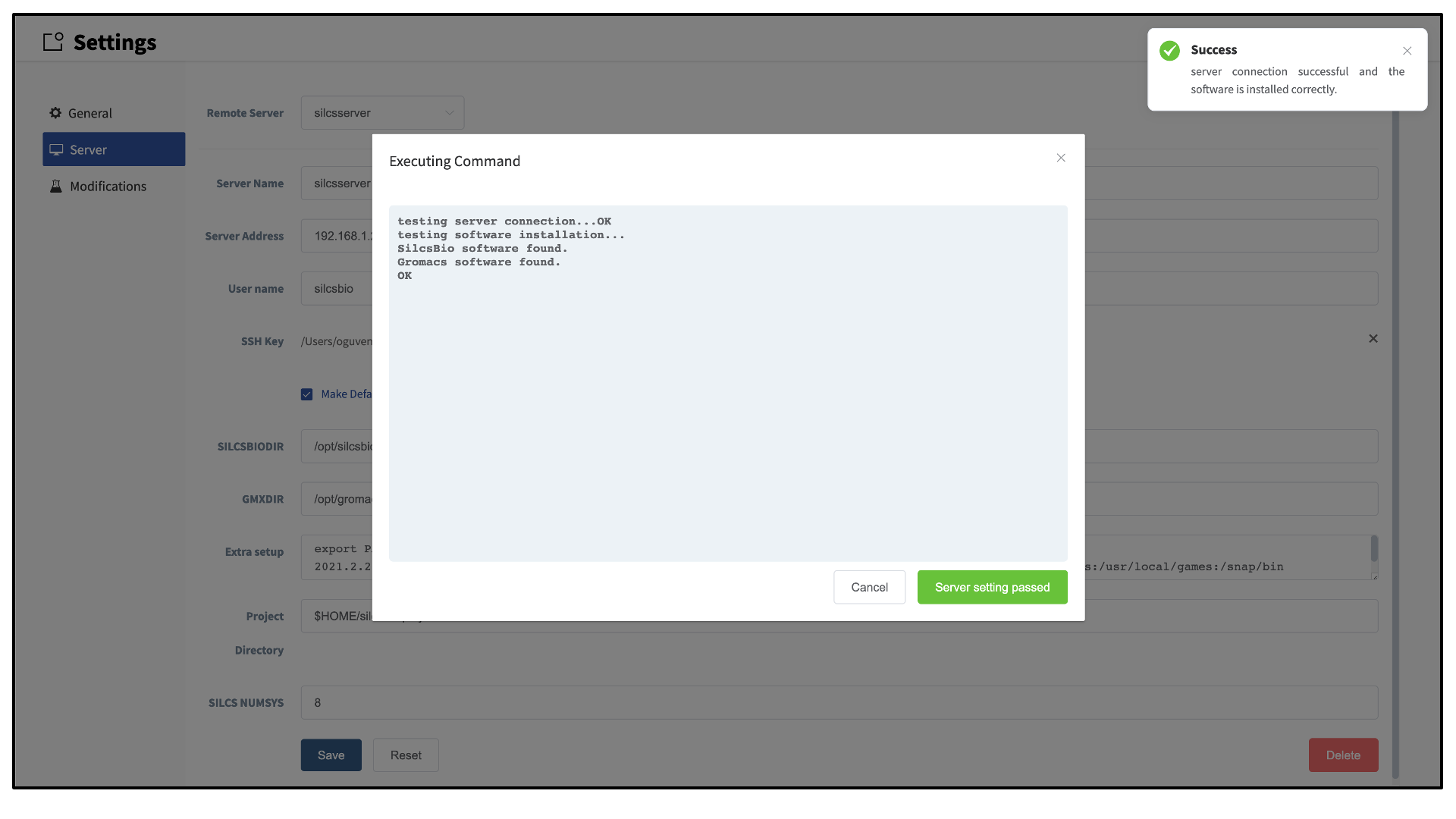
Once all information is entered, click the “Save” button. The GUI will save your entries and confirm that you have a working connection to the server.

Please contact support@silcsbio.com if you need additional assistance.

File and directory selection

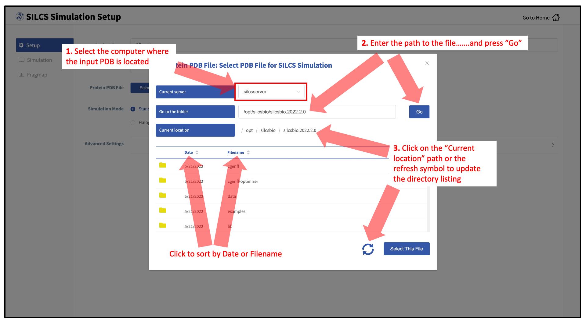
To run the SilcsBio software, you will need to provide protein and/or ligand input files. The SilcsBio GUI has a standardized user interface that allows you to choose these input files from either the computer on which you are running the GUI or from a remote server you have previously configured. Steps to do this, illustrated in the below figure, are as follows.

1. Choose the “Current server,” which is the physical location of the input file. If you would like to load a file located on the computer on which you are running the GUI, select “localhost”; otherwise, select the remote server name of a server you have previously configured through the Remote server setup process.

2. Type in the folder where the file is located using the “Go to the folder” field and then click the associated “Go” button. This will update the “Current location” to this folder. Click on the last portion of the “Current location” path (e.g. “silcsbio.2020.2.0” in “/opt/silcsbio/silcsbio.2020.2.0” in the below example) to update the directory listing located under that path. If you click on any other portion of the “Current location” path, you will be taken to that folder. Double clicking on a folder in the directory listing will move you into that folder.

3. In the directory listing, click on a file to highlight it and click the “Select This File” button at the bottom to finish your file selection.

Follow a similar process to select a directory for those tasks requiring directory selection.

Tip

For those tasks needing FragMaps as inputs, “FragMap Location” needs to be a directory. The SilcsBio GUI assumes a directory path of the form <basename>/maps/. Select <basename> for your “FragMap Location”. The GUI will automatically look for the maps/ subdirectory and load FragMaps from that subdirectory. It will also automatically load the protein pdb file if one is located in the <basename> directory. It may take a few seconds for the GUI to download your input FragMaps if they are not on localhost.

SILCS simulation from the GUI

To begin a new SILCS project, follow these steps:

1. Select New SILCS project from the Home page.

2. Enter a project name and select the remote server where the SILCS jobs will run. Input and output files from the SILCS jobs will be stored on this server based on your choice of “Project Directory” during the Remote server setup process.

   

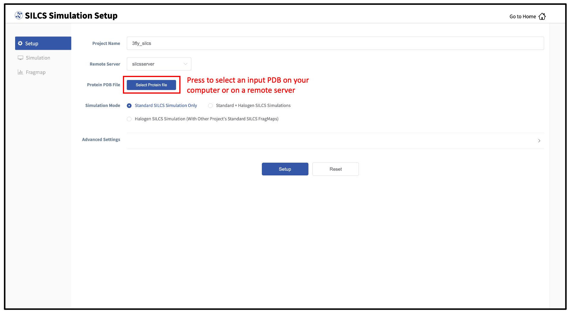
   Next, select a protein PDB file. As described in File and directory selection, choose a file from your local computer (“localhost”) or from any server you had configured through the Remote server setup process. We recommend cleaning your input PDB file before use, incuding keeping only those protein chains that are necessary for the simulation, removing all unnecessary ligands, renaming non-standard residues, filling in missing atomic positions, and, if desired, modeling in missing loops.

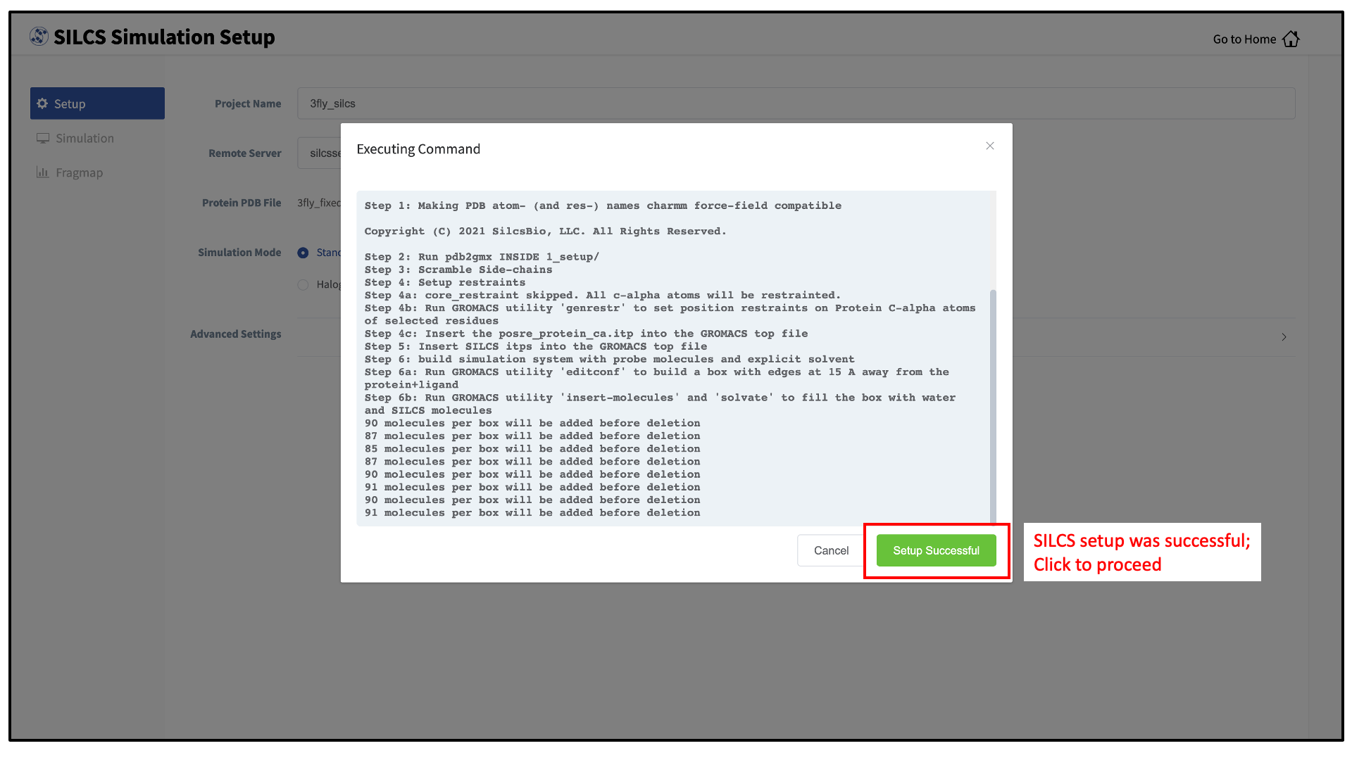
   If the GUI detects missing non-hydrogen atoms, non-standard residue names, or non-contiguous residue numbering, it will inform the user and provide a button labeled “Fix?”. If this button is clicked, a new PDB file with these problems fixed and with _fixed added to the base name will be created and used. Press the “Setup” button at the bottom of the page. The GUI will contact the remote server and perform the SILCS GCMC/MD setup process.

   

3. During setup, the program automatically performs several steps: building the topology of the simulation system, creating metal-protein bonds if metal ions are found, rotating side chain orientations to enhance sampling, and putting probe molecules around the protein. To complete the entire process may take up to 10 minutes depending on the system size. A green “Setup Successful” button will appear once the process has successfully completed. Press this button to go to the next step.

   

4. Your SILCS GCMC/MD simulation can now be started by clicking the “Run SILCS Simulation” button. Before running, you may wish to double check that you have chosen the desired file folder on the remote server and that it has 100+ GB of storage space.

   

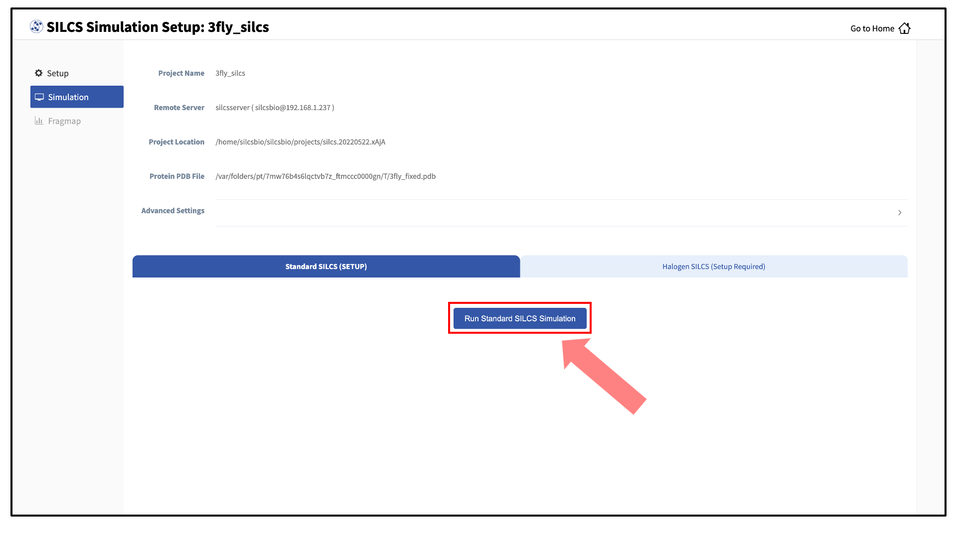
   Compute jobs will be submitted to the queueing system on the server.

   

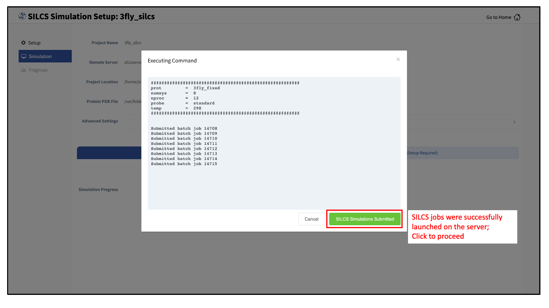
   The status of each job is shown next to its progress bar: “Q” for queued and “R” for running. When a job successfully completes, its progress bar will turn green.

   

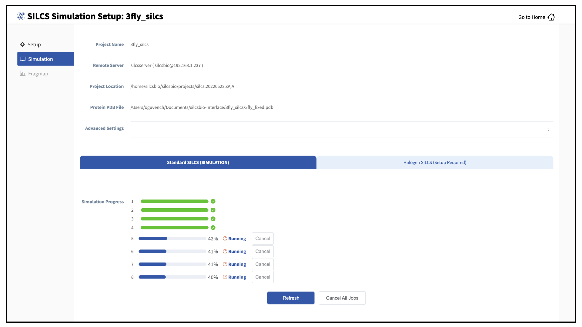
   Once your jobs are in progress, in either the queued or running state, you may safely quit the SilcsBio GUI or go back to the Home page to do other tasks.

   If a job encounters an error or you cancel it before it finishes, its progress bar will turn red. “Restart” will appear next to the progress bar. Pressing “Restart” will resubmit the job to the queue and continue from the last cycle of the calculation so that previous progress on that job is not lost.

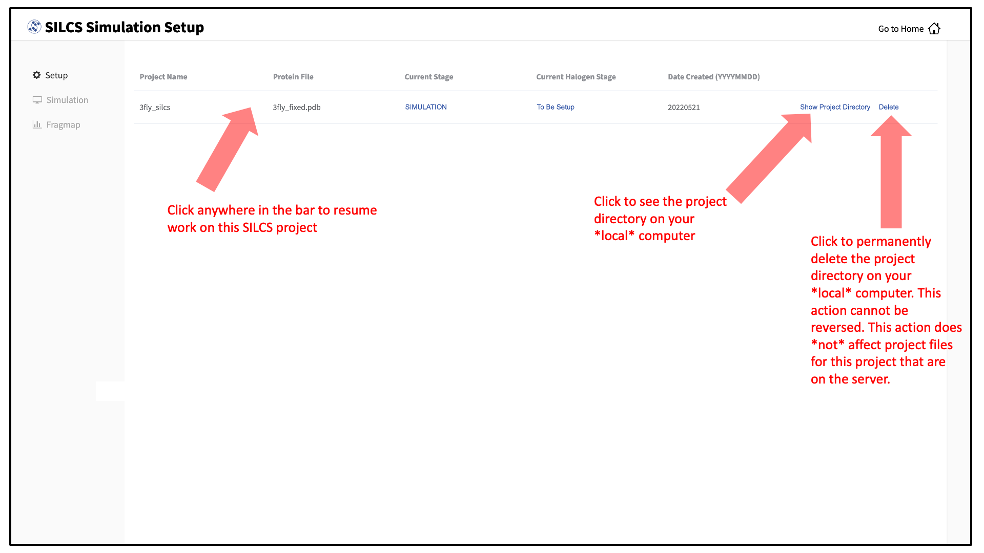
5. To see a full listing of all of your projects, select Continue SILCS project from the Home page. This will show the complete list of all SILCS projects you have set up on the local machine where you are currently running the SilcsBio GUI, as well as the status of each project.

   

   To resume work on a project or check the status of associated compute jobs you previously started, simply click the project name in the list.

   

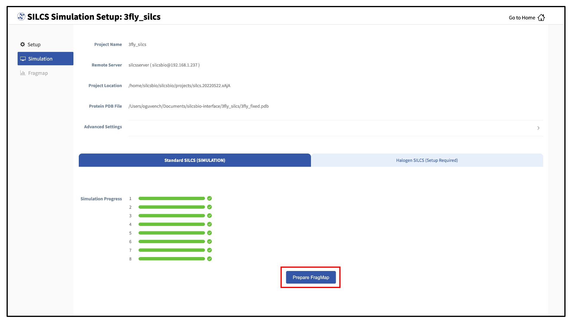
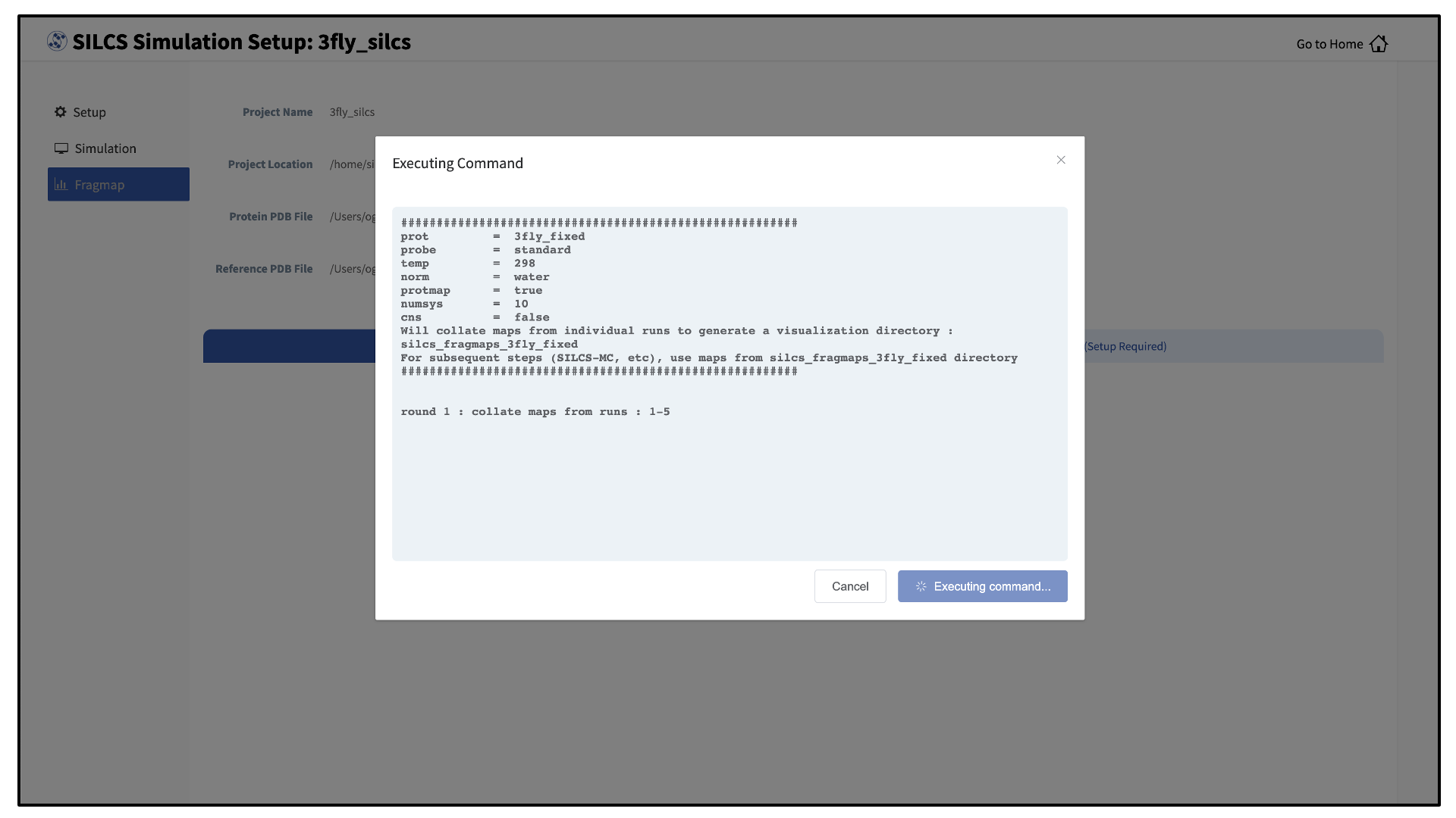
6. Once your SILCS project compute jobs are finished, the GUI can be used to create FragMaps and visualize them. Green progress bars indicate successful job completion. Once all progress bars are green, the “Prepare FragMap” button will appear.

   

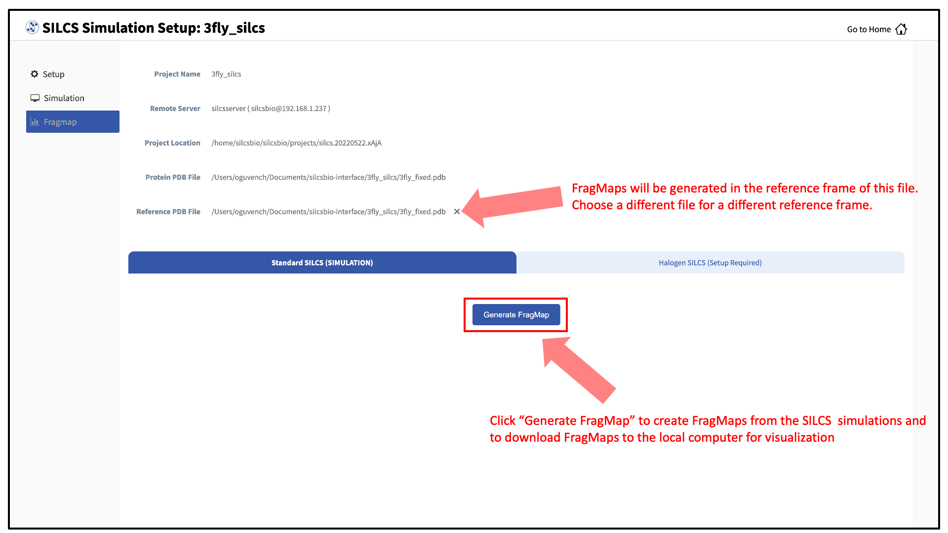
   Press this button, and on the next screen, confirm your “Reference PDB File.” FragMaps will be created in the coordinate reference frame of this file. Generally, this reference PDB file is the same as the protein PDB file. A different file with the protein in a different orientation can be selected if you want to generate FragMaps relative to that orientation. Click “Generate FragMap” to generate FragMaps and download them to the local computer for visualization.

   Tip

   If you plan to compare FragMaps from two different protein structures, you will want to generate them with the same orientation. In that case, pre-align your input structures with each other and use these aligned coordinates as your Reference PDB Files.

   

Processing the GCMC-MD trajectories will take 10-20 minutes, with the GUI providing updates on progress from the server during the process.

Once completed, the GUI will automatically copy the files from the server to the local computer and load them for visualization. Please see Visualizing SILCS FragMaps for details on how to use the SilcsBio GUI, as well as external software (MOE, PyMol, VMD), to visualize SILCS FragMaps.

SILCS FragMaps are the basis for a host of functionality. The FragMaps can be used for optimization of a parent ligand (SILCS-MC: Ligand Optimization), docking of ligands and refinement of existing docked poses (SILCS-MC: Docking and Pose Refinement), creation of pharmacophore models (SILCS-Pharm: Receptor-Based Pharmacophore Models from FragMaps), and detection of hotspots and fragment-based drug design (SILCS-Hotspots: Fragment Binding Sites Including Allosteric Sites).

For additional details on SILCS, please see SILCS: Site Identification by Ligand Competitive Saturation.

SSFEP simulation from the GUI

To begin a new SSFEP project, follow these steps:

1. Select New SSFEP project from the Home page.

2. Enter a project name, and select the remote server where compute jobs will run. Typical SSFEP simulations produce output files in excess of 20 GB, so please select a project location file folder with appropriate storage capacity.

   

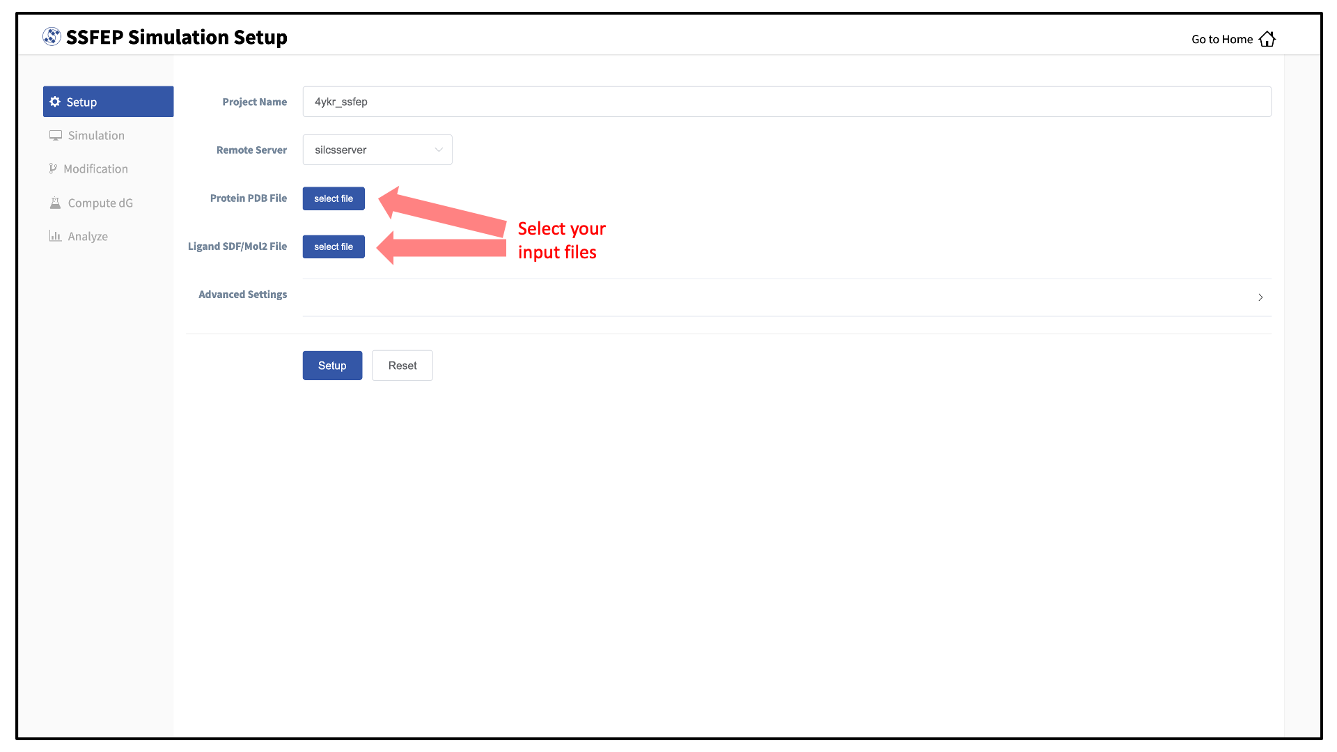
   Next, select a protein PDB file and a ligand file as described in File and directory selection. The ligand should be aligned to the binding pocket in the accompanying protein PDB file. We recommend cleaning your PDB file before use, incuding keeping only those protein chains that are necessary for the simulation, removing all unnecessary ligands, renaming non-standard residues, filling in missing atomic positions, and, if desired, modeling in missing loops.

   If the GUI detects missing non-hydrogen atoms, non-standard residue names, or non-contiguous residue numbering, it will inform the user and provide a button labeled “Fix?”. If this button is clicked, a new PDB file with these problems fixed and with _fixed added to the base name will be created and used in the SSFEP simulation.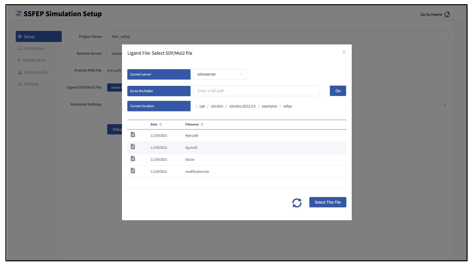

   

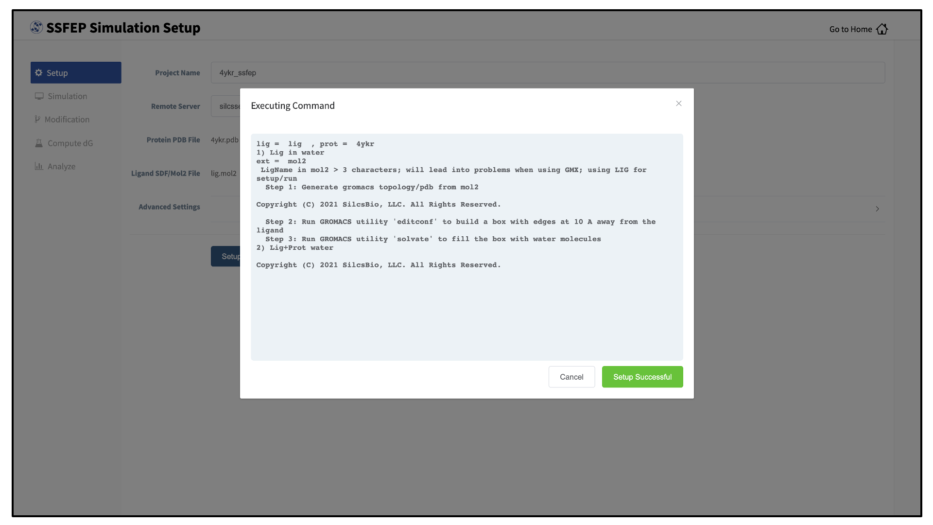
3. Once all information is entered correctly, press the “Setup” button at the bottom of the page. The GUI will contact the remote server and perform the SSFEP setup process.

   During setup, the program automatically performs several steps including building the topology of the simulation system and creating metal-protein bonds if metal ions are found. To complete the entire process may take up to 10 minutes depending on the system size. A green “Setup Successful” button will appear once the process has successfully completed. Press this button to proceed.

   

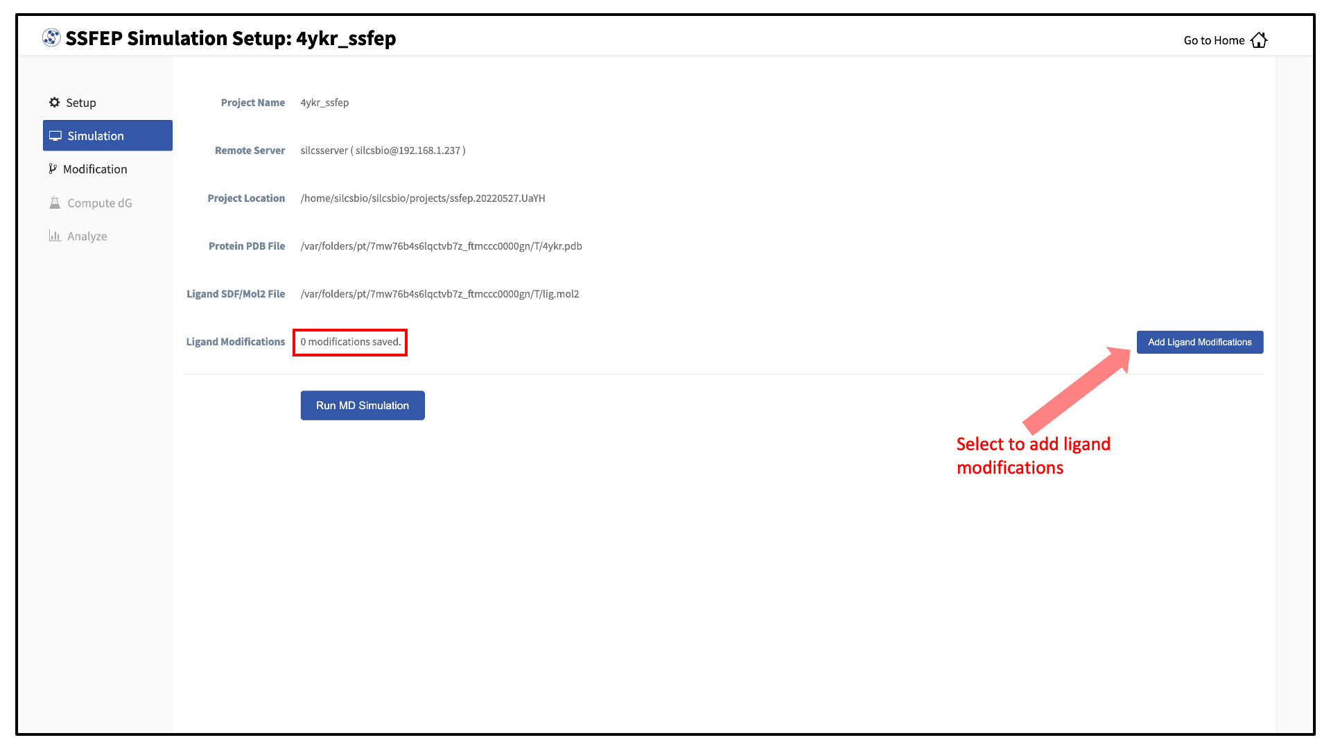
4. You can now prepare your ligand modifications with the “Add Ligand Modifications” button.

   

   There are two major modification types, Substitution and Replacement, available in the GUI. Substitution is used to substitute a hydrogen with another functional group. Replacement is used to replace an atom in a ring with another functional group that preserves the ring.

   In the visualization window, select the atom to be modified. Then, select your desired modifications from the “Substitution” or the “Replacement” tab in the right-hand panel. Pressing the “Save” button in the panel will update your list of modifications.

   

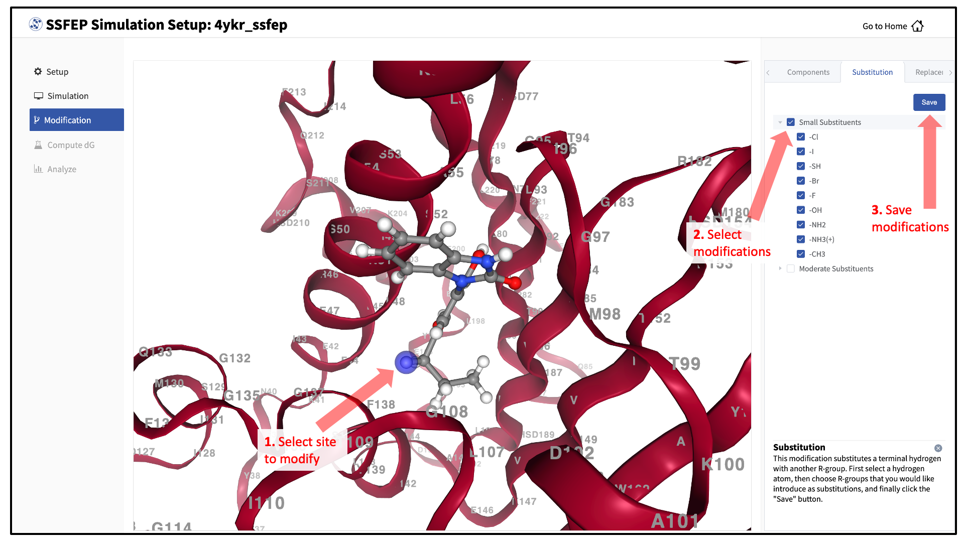
   The list of modification types in the GUI covers a broad range of chemical functionality. Custom modifications can be made using the Command Line Interface (CLI) as detailed in SSFEP: Single Step Free Energy Perturbation.

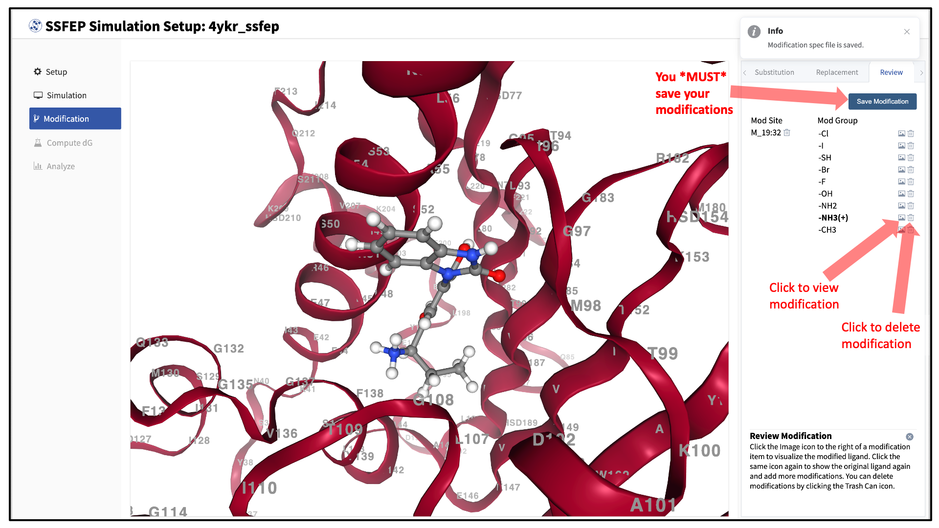
6. Use the “Review” tab to confirm your desired modifications.

   Valid modifications will have a small Image icon as well as a small Trash Can icon. Clicking on the Image icon will show the modification in the center panel. Clicking on it again will show the parent ligand. Clicking on the Trash Can icon will delete the proposed modification from your list. You can go back to the “Substitution” and “Replacement” tabs to add to your list. Once you have completed your list of modifications, you must press the “Save Modification” button in the “Review” tab to actually save the list of modifications for your project.

   

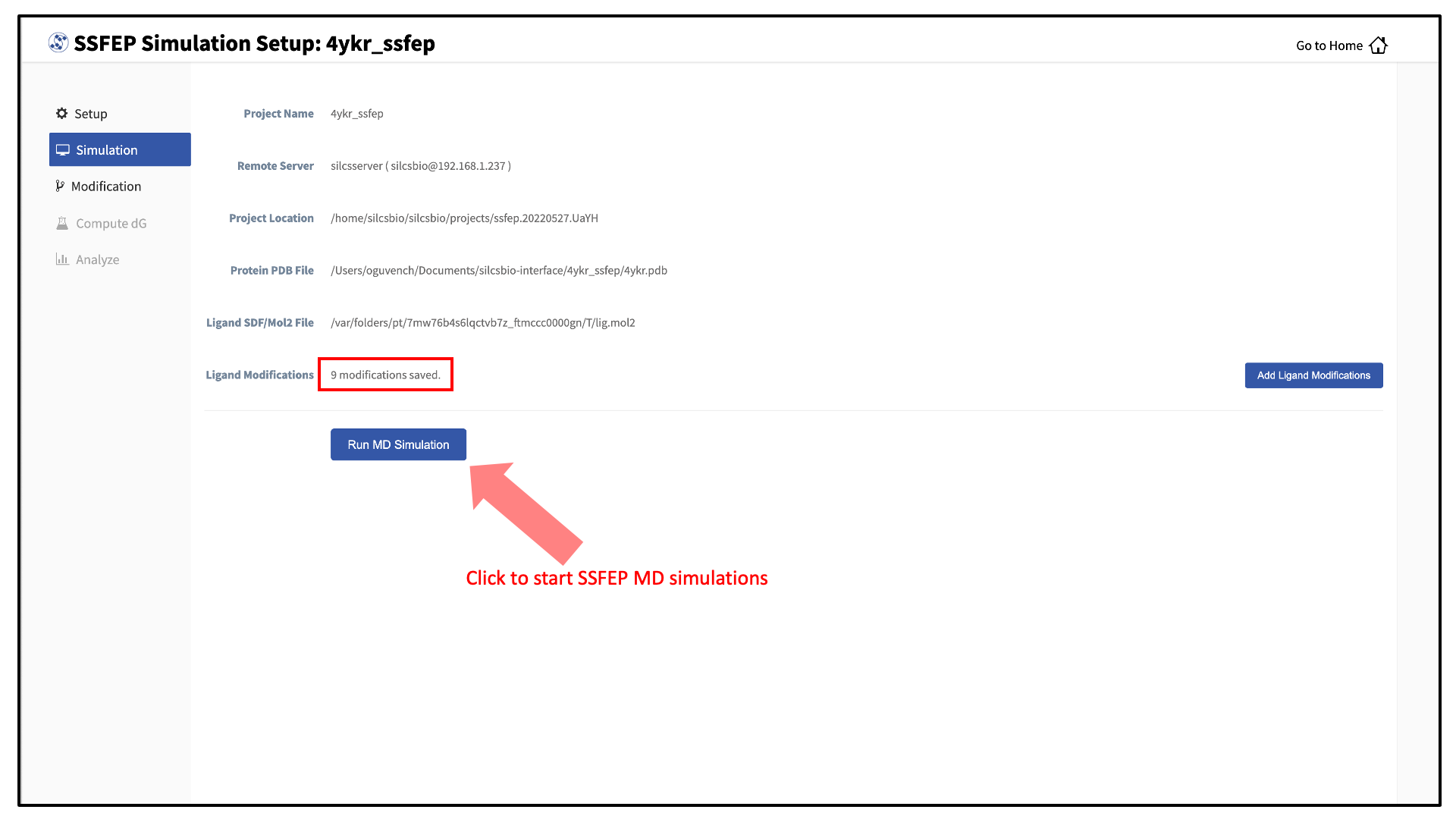
4. Your SSFEP simulation can now be started by selecting “Simulation” from the left-hand pane and then clicking the “Run MD Simulation” button in the resulting screen. Before running, you may wish to double check that you have chosen the desired file folder on the remote server and that it has 20+ GB of storage space. There are two parts to SSFEP: a compute-intensive MD simulation and a very rapid \(\Delta \Delta G\) calculation. The compute-intensive MD may take several hours, and is done only once. The rapid \(\Delta \Delta G\) calculation part relies on the MD results and is able to test thousands of functional group modifications to your parent ligand in under an hour. Should you wish to test additional modifications to your parent ligand at a later time in the project, there is no need to re-run the compute-intensive MD, which makes SSFEP a very efficient method.

   

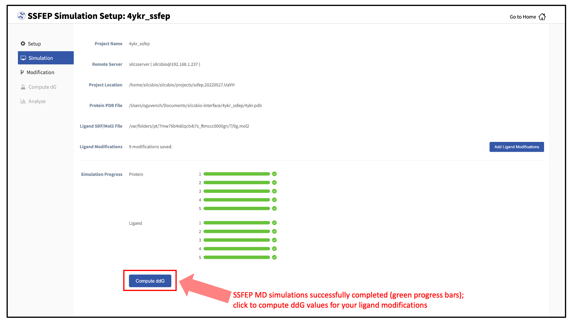
   10 compute jobs will be submitted to the queueing system (five for the ligand and five for the protein:ligand complex) on your remote server. Job progress will be displayed in this same window. The status of each job is shown next to its progress bar: “Q” for queued and “R” for running, At this point, your jobs are in progress and you may safely quit the SilcsBio GUI or go back to the Home page to do other tasks.

   If a job encounters an error and does not finish, a “restart” button will appear next to the status. If the restart button is used, the job will be resubmitted to the queue and continue from the last cycle of the calculation.

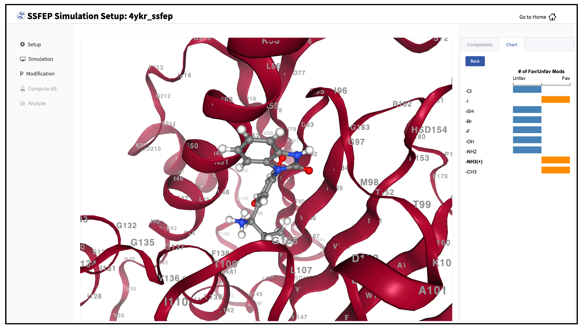
8. Once the MD simulation stage has finished, use the GUI to automatically analyze your list of modifications and create a chart.

   

   SSFEP is designed to evaluate small modifications and results are best interpreted qualitatively. Therefore GUI-created charts indicate the predicted change in direction of the binding affinity relative to the parent ligand.

   

For additional details on SSFEP, please see SSFEP: Single Step Free Energy Perturbation.