Site Identification by Ligand Competitive Saturation (SILCS)

Background

The design of small molecules that bind with optimal specificity and affinity to their biological targets, typically proteins, is based on the idea of complementarity between the functional groups in a small molecule and the binding site of the target. Traditional approaches to ligand identification and optimization often employ the one binding site/one ligand approach. While such an approach might be straightforward to implement, it is limited by the resource intensive nature of screening and evaluating the affinity of large numbers of diverse molecules.

Functional group mapping approaches have emerged as an alternative, in which a series of maps for different classes of functional groups encompass the target surface define the binding requirements of the target. With such maps in hand, medicinal chemists can focus their efforts on designing small molecules that best match the maps.

Site Identification by Ligand Competitive Saturation (SILCS) offers rigorous free energy evaluation of functional group affinity pattern for the entire 3D space in and around a protein [3]. The SILCS method yields functional group free energy maps, or FragMaps, which are precomputed and rapidly used in a variety of ways to facilitate ligand design. FragMaps are generated by molecular dynamics (MD) simulations that include protein flexibility and explicit solvent/solute representation, thus providing an accurate, detailed, and comprehensive collection of information that can be used qualitatively in database screening, fragment-based drug design and lead optimization.

In addition, in the context of biological therapeutics, the comprehensive nature of the FragMaps is of utility for excipient design as all possible binding sites of all possible excipients and buffers can be identified and quantified.

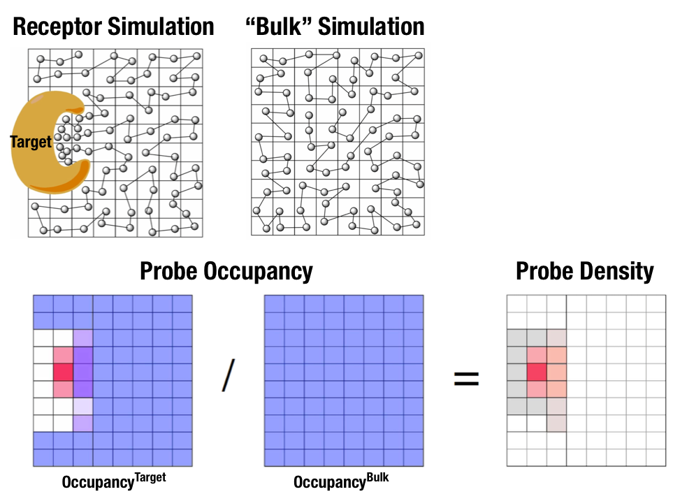
Fig. 1 Illustration of fragment density maps.

Fig. 1 illustrates FragMaps generation. Two MD simulations of a probe molecule (e.g., benzene) are performed in the presence of a protein and in aqueous solution (without protein), resulting in two occupancy maps, \(O^\mathrm{target}\) and \(O^\mathrm{bulk}\), respectively. The GFE (grid free energy) FragMaps are then derived by the following formula

\[\mathrm{GFE}^T_{x,y,z} = -RT \log \frac{O^\mathrm{target}_{x,y,z}}{\left< O^\mathrm{bulk} \right>}\]

By generating FragMaps using various small solutes representing different functional groups including benzene, propane, methanol, imidazole, formamide, acetaldehyde, methylammonium, acetate, and water, it is possible to map the functional group affinity pattern of a protein. FragMaps encompass the entire protein such that all FragMap types are in all regions. Thus, information on the affinity of all the different types of functional groups is available in and around the full 3D space of the protein or other target molecule.

FragMaps may be used in a qualitative fashion to facilitate ligand design by allowing the medicinal chemist to readily visualize regions where the ligand can be modified or functional groups added to improve affinity and specificity. As the FragMaps include protein flexibility, they indicate regions of the target protein that can “open” thereby identifying regions under the protein surface accessible for ligand binding. In addition to FragMaps, an “exclusion map” is generated based on regions of the system that are not sampled by water or probe molecules during the MD simulations. The exclusion map represents a strictly inaccessible surface.

Many proteins contain binding sites that are partially or totally inaccessible to the surrounding solvent environment that may require partial unfolding of the protein for ligand binding to occur. SILCS sampling of such deep or inaccessible pockets is facilitated by the use of a Grand Canonical Monte Carlo (GCMC) sampling technique in conjunction with MD simulations [4]. Thus, the SILCS technology is especially well suited for ligand design pockets targeting the deep and inaccessible binding sites found in GPCRs, nuclear receptors and so on.

Once a set of ligand-independent SILCS FragMaps are produced they may be rapidly used for various purposes that quantitatively rank ligand binding in a highly computationally efficient manner for multiple ligands WITHOUT recalculating the FragMaps. Applications of SILCS methodology include:

• Binding site identification
  • Binding pocket searching with known ligands
  • Binding pocket identification via pharmacophore generation
  • Binding pocket identification via fragment screening
• Database screening
  • SILCS 3D pharmacophore models
  • Ligand posing using available techniques (Catalyst, etc)
  • Ligand ranking
• Fragment-based ligand design
  • Identification of fragment binding sites
  • Estimation of ligand affinity following fragment linking
  • Expansion of fragment types
• Ligand optimization
  • Qualitative ligand optimization by FragMaps visualization
  • Quantitative evaluation of ligand atom contributions to binding
  • Quantitative estimation of relative ligand affinities
  • Quantitative estimation of large numbers of ligand chemical transformations
• Ligand optimization can also be performed via rapid free energy perturbations of small functional group transformations via the SSFEP technology (see the SilcsBio SSFEP Users Guide).

SILCS generates 3D maps of interaction patterns of functional group with your target molecule, called FragMaps. This unique approach simultaneously uses multiple small solutes with various functional groups in explicit solvent MD simulations that include target flexibility to yield 3D FragMaps’ that represent the delicate balance of target-functional group interactions, target desolvation, functional group desolvation and target flexibility. The FragMaps may then be used to both qualitatively direct ligand design and quantitatively to rapidly evaluate the relative affinities of large numbers of ligands following the computationally demanding precomputation of the FragMaps.

In this document, we will go over the workflow of generating the FragMaps, and how to visualize them.

Running SILCS Simulations Using a Graphical User Interface

To generate the FragMaps, a well-curated protein structure file (without ligand) is required in PDB file format. The protein structure should have termini properly capped, missing loops built or the ends of the missing loops capped, the proper protonation states assigned and so on. Please inquire if assistance with protein preparation is required.

Setup FragMap Simulation

Select New SILCS project button from the landing page. This will take you to the new project setup page.

Enter a project name, select remote server, and select project location from the remote server. The project location is where the SILCS simulation will be performed. Typical SILCS simulation may produce output file size more than 100 GB, so please select the folder with a large storage volume.

Next, select a protein PDB file. We recommend clean up PDB before using in SILCS simulation, such as only keeping the chains that are necessary for the simulation, removing any unnecessary ligands, renaming non-standard residues, and filling in the missing atomic positions.

If the interface detects missing heavy atoms, non-standard residue name, or non-contiguous residue numbering, it will inform the user and provide a button labeled as “Fix?”. If this button is clicked, a new PDB file with “_fixed” suffix will be created and used in the SILCS simulation.

Once all the information is entered correctly, press “Setup” button at the bottom of the page. The interface will contact the remote server and perform SILCS GCMC/MD setup process.

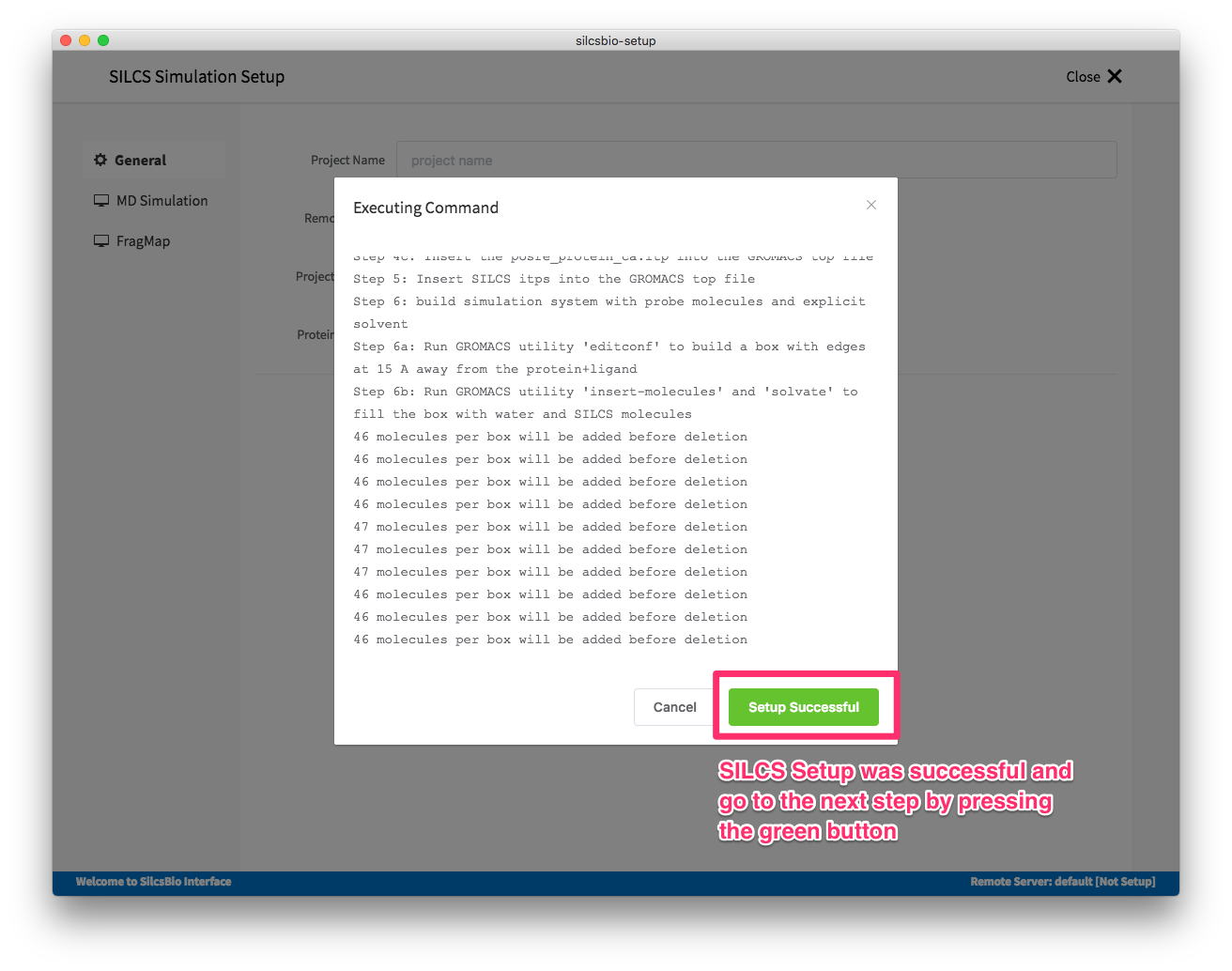
During this step, the program performs several steps under the hood; building the topology of the simulation system, creating metal-protein bond if metal ions found, perturb side chain orientations for enhancing sampling, and putting probe molecules around the protein. These process may take up to 5-10 minutes depending on the system size.

After confirming the setup is finished, please make sure information entered are correct and the remote project location has an ample storage space. When it is ready, SILCS GCMC/MD simulation can be started by clicking the “Run SILCS Simulation” button.

This will submit 10 jobs to the queue system. The progress of the jobs will be displayed on the same page. The status of the job is also shown next to the progress bar; “Q” for being in the queue, “R” for running, and “E” for finished.

Generate FragMaps

Once the simulation is finished, the GUI will help the user to create FragMap and visualize them.

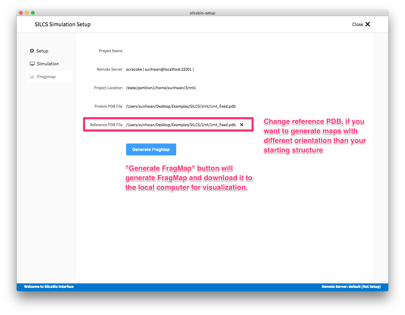
In case you want to compare the maps from two different protein structures, you may want to generate maps with the same orientation. In that case, pre-align the inputs structures with the another and use the aligned structure in the reference PDB file.

This command will merge the occupancy maps from individual runs and create a GFE FragMaps. The following maps will be generated under silcs_fragmap_<protein PDB>/maps directory. The PyMOL and VMD scripts that loads those maps will also be created under silcs_fragmap_<protein PDB> folder.

Running SILCS Simulations using Command Line Interface

To generate the FragMaps, a well-curated protein structure file (without ligand) is required in PDB file format. The protein structure should have termini properly capped, missing loops built or the ends of the missing loops capped, the proper protonation states assigned and so on. Please inquire if assistance with protein preparation is required.

Setup FragMap Simulation

${SILCSBIODIR}/silcs/1_setup_silcs_boxes prot=<Protein PDB>

Warning

The setup program internally uses the GROMACS utility pdb2gmx, which may have problems processing the protein PDB file. The most common reasons for errors at this stage involve mismatches between the expected residue name/atom names in the input PDB and those defined in the CHARMM force-field.

To fix this problem: Run the pdb2gmx command manually from within the 1_setup directory for a detailed error message. The setup script already prints out the exact commands you need to run to see this message.

cd 1_setup pdb2gmx –f <PROT PDB NAME>_4pdb2gmx.pdb –ff charmm36 –water tip3p –o test.pdb –p test.top -ter -merge all

Once all the errors in the input PDB are corrected, rerun the setup script.

Following completion of the setup, run 10 GCMC/MD jobs using the following script:

${SILCSBIODIR}/silcs/2a_run_gcmd prot=<Protein PDB>

This script will submit 10 jobs to the predefined queue. Each job runs out 100 ns of GCMC/MD with the protein and the solute molecules.

Once the simulations are complete, the 2a_run_gcmd/[1-10] directories will contain *.prod.125.rec.xtc trajectory files. If these files are not generated, then your simulations are either still running, or stopped due to some problem. Look into the log files within these directories for an explanation of the failure.

Generate FragMaps

Once your simulations are done, generate the FragMaps using the following script.

${SILCSBIODIR}/silcs/2b_gen_maps prot=<Protein PDB>

This script will submit 10 single-core jobs. These will build occupancy maps spanning the simulation box for selected solute molecule atoms representing different functional groups. For a ~50K atom simulation system, this job takes approximately 10-20 minutes to complete. The FragMaps have a default spacing of 1 Å. This grid spacing can be changed by providing the parameter spacing=<grid spacing in Å>.

Warning

A smaller grid spacing than 1 Å may make FragMpas more noisy and may require a longer simulation or smoothing of maps (postprocessing).

Next, issue the following command to combine the occupancy maps generated from individual simulations and convert them into GFE FragMaps. Each voxel in the map file contains Grid Free Energy (GFE) for the solute atoms.

${SILCSBIODIR}/silcs/2c_fragmap prot=<Protein PDB>

This command will merge the occupancy maps from individual runs and create a GFE FragMaps. The following maps will be generated under silcs_fragmap_<protein PDB>/maps directory. The PyMOL and VMD scripts that loads those maps will also be created under silcs_fragmap_<protein PDB> folder.

<prot name>.benc.gfe.map    Aromatic map
<prot name>.prpc.gfe.map    Aliphatic map
<prot name>.aceo.gfe.map    Charged acceptor map
<prot name>.mamn.gfe.map    Charged donor map
<prot name>.forn.gfe.map    Polar nitrogen donor map (Formamide)
<prot name>.foro.gfe.map    Polar oxygen acceptor map (Formamide)
<prot name>.imin.gfe.map    Polar nitrogen acceptor map (Imidazole)
<prot name>.iminh.gfe.map   Polar nitrogen donor map (Imidazole)
<prot name>.aalo.gfe.map    Polar oxygen acceptor map (Acetaldehyde)
<prot name>.meoo.gfe.map    Polar oxygen acceptor map (Methanol)
<prot name>.apolar.gfe.map  Generic Apolar maps
<prot name>.hbdon.gfe.map   Generic donor maps
<prot name>.hbacc.gfe.map   Generic acceptor maps
<prot name>.excl.map        Exclusion map
<prot name>.ncla.map        Zero map

Clean up

The raw trajectory file are quite large. To conserve storage usage, hydrogen atom positions can be deleted via using the following command:

${SILCSBIODIR}/silcs/2d_cleanup prot=<Protein PDB>

Setup FragMap Simulation with halogen probe

Halogen probe molecules are supported starting from the version 2018.1 as a beta release. If enabled, 8 probe molecules (bromobenzene, chlorobenzene, chloroethane, dimehtylether, fluoroethane, fluorobenzene, methanol, trifluoroethane) will be used instead of the standard ones.

To setup and run SILCS simulation with halogen probes, add halogen=true in each command. For example, use the following commands to setup SILCS simulation, run GCMC/MD simulation, and compute FragMaps.

${SILCSBIODIR}/silcs/1_setup_silcs_boxes prot=<Protein PDB> halogen=true
${SILCSBIODIR}/silcs/2a_run_gcmd prot=<Protein PDB> halogen=true
${SILCSBIODIR}/silcs/2c_fragmap prot=<Protein PDB> halogen=true

The directory structure stays the similar to the standard simulation, but uses _x suffix in each of the directories. For example, the SILCS simulation setup will be kept under 1_setup_x folder (instead of 1_setup as in standard SILCS probe simulation). Similarly, the GCMC/MD simulation and FragMap will be kept under 2a_run_gcmd_x and 2b_gen_maps_x folder.

Halogen probe SILCS simulation is currently at a beta stage, and we expect some steps may result in error. If you encounter a problem, please let us know and we will help/fix the problem.

Setup FragMap Simulation with GPCR targets

Running SILCS simulations with GPCR targets are supported starting from the version 2018.1 as a beta release. The GPCR target is currently limited to simulation standard probe (no halogen probe support) in the current version.

The command line utility that builds protein/membrane complex is provided. In the current version, the choice of membrane is limited to 9:1 POPC/Chol mixture. Use the following command to insert protein into the bilayer.

${SILCSBIODIR}/silcs-memb/1a_fit_protein_in_bilayer prot=<Protein PDB>

This command line utility will use the first principal axis to the membrane normal (Z-axis) and translate the center of the mass to the center of the membrane bilayer (Z=0).

If the protein is already oriented in membrane, use orient_principal_axis=false keyword to suppress principal axis-based orientation.

${SILCSBIODIR}/silcs-memb/1a_fit_protein_in_bilayer prot=<Protein PDB> orient_principal_axis=false

By default the system size is set to 120 Å along the X and Y. To change the size of the system, use bilayer_x_size and bilayer_y_size option.

${SILCSBIODIR}/silcs-memb/1a_fit_protein_in_bilayer prot=<Protein PDB> bilayer_x_size=<X dimension> bilayer_y_size=<Y dimension>

The output produced the above command line utility is the protein structure embedded in a POPC/Chol 9:1 mixed bilayer and have a suffix of _popc_chol to the input PDB filename. The correct orientation and the size of the membrane should be confirmed to ensure protein is properly embedded in the membrane.

To prepare SILCS simulation box, use the following command line utility:

${SILCSBIODIR}/silcs/1b_setup_silcs_in_bilayer prot=<Protein/bilayer PDB>

This will add water and probe molecules to the system. If for various reason, orientation from 1a_fit_protein_bilayer did not correctly orient the protein into the bilayer, a custom protein/membrane complex can be used to prepare the input PDB and be used as an input for 1b_setup_silcs_in_bilayer utility.

Finally, the SILCS GCMC/MD simulation can be performed using the following command:

${SILCSBIODIR}/silcs-memb/2a_run_gcmd prot=<Protein/bilayer PDB>

This will perform SILCS GCMC/MD simulation with a slightly modified protocol. Briefly, a 6-step pre-equilibration relaxing the bilayer slowly, followed by 10 ns of relaxation of protein into the bilayer before production without restraint potential. Please note that GPCR simulation systems are typically large and may require significant storage space (> 200 GB) and longer simulation time (~15 days with GPUs).

The FragMap generation is independent of membrane, so the same SILCS command line utility, such as $SILCSBIODIR/silcs/2b_gen_maps and $SILCSBIODIR/silcs/2c_fragmap can be used to produce FragMaps.

SILCS GPCR simulation is currently at a beta stage, and we expect some steps may result in error. If you encounter a problem, please let us know and we will help/fix the problem.

Visualizing FragMaps

GFE FragMaps will be stored in the directory 2b_gen_maps. This folder contains the specific and generic FragMaps indicated above. FragMaps are defined based on non-hydrogen atoms. For certain solute types there are multiple FragMaps (imidazole, formamide). FragMaps for water oxygens (tipo) are included to identify water molecules that are difficult to displace. Generic FragMaps for apolar (benzene, propane), H-bond donor (neutral H-bond donors) and H-bond acceptor (neutral H-bond acceptors) probe types are included to simplify visualization.

For easy visualization, we provide plugins for the visualization softwares VMD and PyMOL.

FragMaps in VMD

To visualize the maps in VMD, use the plugins provided. First, load the protein structure used in FragMap generation onto VMD. Once the protein structure is loaded, select Extensions ‣ SilcsBio ‣ FragMap Tools to activate the plugin window. If the plugin is not yet installed, see VMD plugin installation for the instruction.

Fig. 2 VMD FragMap Plugin

The “map folder” is the name of folder that contains FragMap files, which is typically “2b_gen_maps”. The “map prefix” is the protein PDB name used when setting up and performing the SILCS simulations. If a protein PDB file was loaded onto VMD prior to opening the plugin window, the name of the PDB file will be taken as a default for this parameter. Once these two parameters are confirmed, select “Visualize FragMap” button at the bottom of the window.

This will load various FragMaps onto the VMD main window, and display a new tab in the plugin window. This new tab allows the user to quickly enable/disable FragMap display using the checkboxes on the left hand side of the window. By default, FragMaps are displayed at -1.2 kcal/mol. This level can be changed by using either +/- buttons or slider.

FragMaps in PyMOL

To visualize the maps in PyMOL, use the plugins provided. First, load the protein structure used in FragMap generation onto PyMOL. Once the protein structure is loaded, select Plug ‣ FragMap Tools to activate the plugin window. If the plugin is not installed, see PyMOL plugin installation for the install instruction.

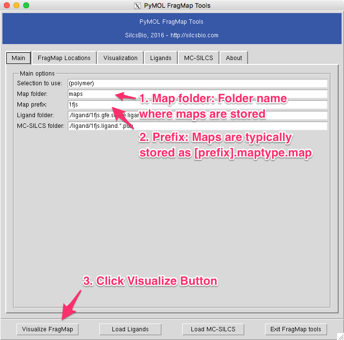
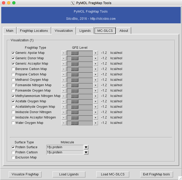
Fig. 3 PyMOL FragMap Plugin

The “map folder” is the name of folder that contains FragMap files, which is typically “2b_gen_maps”. The “map prefix” is the protein PDB name used building FragMap setup. If a protein PDB file was loaded onto PyMOL prior to opening the plugin window, the name of the PDB file will be taken as a default for this parameter. Once these two parameters are confirmed, select “Visualize FragMap” button at the bottom of the window.

This will load various FragMaps onto PyMOL main window, and display a new tab in the plugin window. This new tab allows quickly enable/disable FragMap display using the checkboxes on the left hand side of the window. By default, FragMaps are displayed at -1.2 kcal/mol with an exception of exclusion map. This level can be changed by using left or right arrows on either side of the numeric level indicator.