Usage
In principle, SILCS-Biologics can be applied to any protein therapeutic. In practice, because SILCS is an all-atom explicit-solvent molecular dynamics methodology, the SILCS simulations underpinning SILCS-Biologics can become computationally prohibitive for large proteins, like full-sequence antibodies or non-antibody protein therapeutics of large size. To enable application of SILCS-Biologics to larger proteins, you may split your full protein into two or three domains. SILCS-Biologics will automatically take care of managing the separate SILCS simulations for each domain and the subsequent SILCS-Hotspots and SILCS-PPI analyses, as well as collating the separate data into a single report for the full-length protein. The usage of SILCS-Biologics with the SilcsBio GUI and the CLI is described below. It is strongly recommended that users read and understand the descriptions of the use cases before using either the command line or the SilcsBio GUI to run SILCS-Biologics.
SILCS-Biologics Using the SilcsBio GUI
Please see SILCS-Biologics Using the GUI in the Graphical User Interface (GUI) Quickstart for instructions on running SILCS-Biologics from the SilcsBio GUI.
SILCS-Biologics Using the CLI
The SILCS-Biologics workflow can be run using the following command:
$SILCSBIODIR/silcs-biologics/silcs-biologics step=<1*2*3*4*> prot1=<protein PDB>
Required parameter:
Tasks to be completed:
step=<1*2*3*4*>
All tasks can be submitted at once with a single command with
step=1*2*3*4*. To submit specific tasks or subtasks one step at a time, specify the task by entering only the desired task (e.g.,step=1*to submit only the first task). The tasks and subtasks are listed below:step=1*2*3*4*orstep=1abc2ab3ab4ab: Run all stepsstep=1*: Run SILCS simulations and generate FragMapsstep=1a: set up SILCS simulationsstep=1b: run SILCS simulationsstep=1c: generate FragMaps
step=2*: Run SILCS-PPI (predict protein aggregation sites)step=2a: Run protein–protein docking simulations with SILCS-PPIstep=2b: Collect SILCS-PPI data
step=3*: Run SILCS-Hotspots (predict excipient binding sites)step=3a: Dock excipients onto the target protein with SILCS-Hotspotsstep=3b: Cluster docked poses from SILCS-Hotspots
step=4*: Generate SILCS-Biologics reportstep=4a: Generate web reportstep=4b: Generate spreadsheet report
Path and name of protein PDB file:
prot1=<protein PDB>
Optional parameters:
Path and name of second protein domain PDB file:
prot2=<protein 2 PDB>
The target protein may be divided into domains for computational expediency. In this case, each domain is input as a separate PDB file. For a two domain system,
prot1will correspond to one domain, andprot2will correspond to the remaining domain. For a three domain system,prot1will correspond to the first domain,prot2will correspond to the second domain, andprot3will correspond to the third domain. Ifprot2or bothprot2andprot3are used,fullpdbmust also be specified (see below).Path and name of third protein domain PDB file:
prot3=<protein 3 PDB>
The target protein may be divided into domains for computational expediency. In this case, each domain is input as a separate PDB file. For a three domain system,
prot1will correspond to the first domain,prot2will correspond to the second domain, andprot3will correspond to the third domain. Ifprot2andprot3are used,fullpdbmust also be specified (see below).Path and name of full-length protein PDB file (required if more than one protein is input):
fullpdb=<full-length protein PDB>
If
prot2or bothprot2andprot3are used, then the full-length protein PDB file must also be specified withfullpdb.Note
If you do not have the full-length structure of the target protein, but only have the structures of individual domains, then the full-length protein structure should be constructed using other molecular modeling tools (such as homology modeling software). The modeled full-length structure can then be used as the “Reference PDB File”.
Alternatively, the positions of the individual domains in the context of the full-length protein can be estimated through a simple structural alignment to a known full-length homologous crystal structure, and the resulting superimposed structure of the individual domains can be saved and used as the “Reference PDB File”.
Warning
Dividing the target protein into domains entails independent SILCS simulations for each of the domains. E.g., for SILCS-Biologics runs with
prot1,prot2, andprot3specified (3 domains) 3 \(\times\) 10 SILCS simulations will be performed rather than 1 \(\times\) 10 SILCS simulations. If sufficient compute nodes are available to run all SILCS simulations for all domains simultaneously, the SILCS simulations for the target protein will be completed sooner using the domain approach than running SILCS simulations of the full-length protein. However, using the domain approach may consume more CPU/GPU hours.Path and name of directory containing excipient Mol2/SD files:
molsdir=<directory of the excipient files; default=$SILCSBIODIR/data/excipients/mols>
The excipient structure files in the
molsdirdirectory may be in Mol2 or SD file format. In both formats, only one excipient per file will be read.Tip
If you have a single SD file containing multiple excipients, you may split the file into multiple SD files with one excipient per file using the following command, where
<multiple.sdf>is the SD file containing multiple excipients and<molsdir>is the directory in which all output SD files containing one excipient per file will be placed:${SILCSBIODIR}/programs/format_convertor --split --inf <multiple.sdf> --outf <molsdir>Path and name of buffer molecule Mol2/SD file:
buffer=<path and name of buffer molecule; default="NONE">
Only one buffer molecule can be specified at a time. The buffer molecule file may be in Mol2 or SD file format. In both formats, only one excipient per file will be read. The buffer molecule file can be located in a different directory than
molsdir.ID for the job:
job_id=<id for the current job; default=$jobTime (timestamp)>
Path and name of project working directory:
workdir=<directory of the project; default=$PWD>
Name of directory for first task (step 1):
dir1=<directory for step 1; defaul=$workdir/1_fragmap.$job_id>
Name of directory for second task (step 2):
dir2=<directory for step 2; defaul=$workdir/2_ppi.$job_id>
Name of directory for third task (step 3):
dir1=<directory for step 3; defaul=$workdir/3_excipients.$job_id>
Name of directory for fourth task (step 4):
dir4=<directory for step 4; defaul=$workdir/4_report.$job_id>
Viewing Step 4 Reports
Once all four steps have completed, reports will be ready for viewing and analysis.
Tip
If you ran your SILCS-Biologics workflow using the SilcsBio GUI, these reports will also be available for viewing via the SilcsBio GUI. Please refer to SILCS-Biologics Using the GUI for more information.
Viewing through a Spreadsheet Application
If you wish to open these data in a spreadsheet application, you can
find them in $WORKDIR/4_report.$job_id/,
where $WORKDIR is the top-level directory containing all the
silcs-biologics workflow outputs. By default, $job_id is set
based on the system date and time, and $WORKDIR is set to the directory
in which the silcs-biologics command was executed. You can override
these defaults with the options job_id= and workdir= when
executing silcs-biologics.
Tip
See SILCS-Biologics Directory Structure for a complete
description of how silcs-biologics organizes and names the
directories and files that it creates.
$WORKDIR/4_report.$job_id/report_all.xlsx has a tab named “Ranking”
that contains a number of properties on a per-excipient basis:
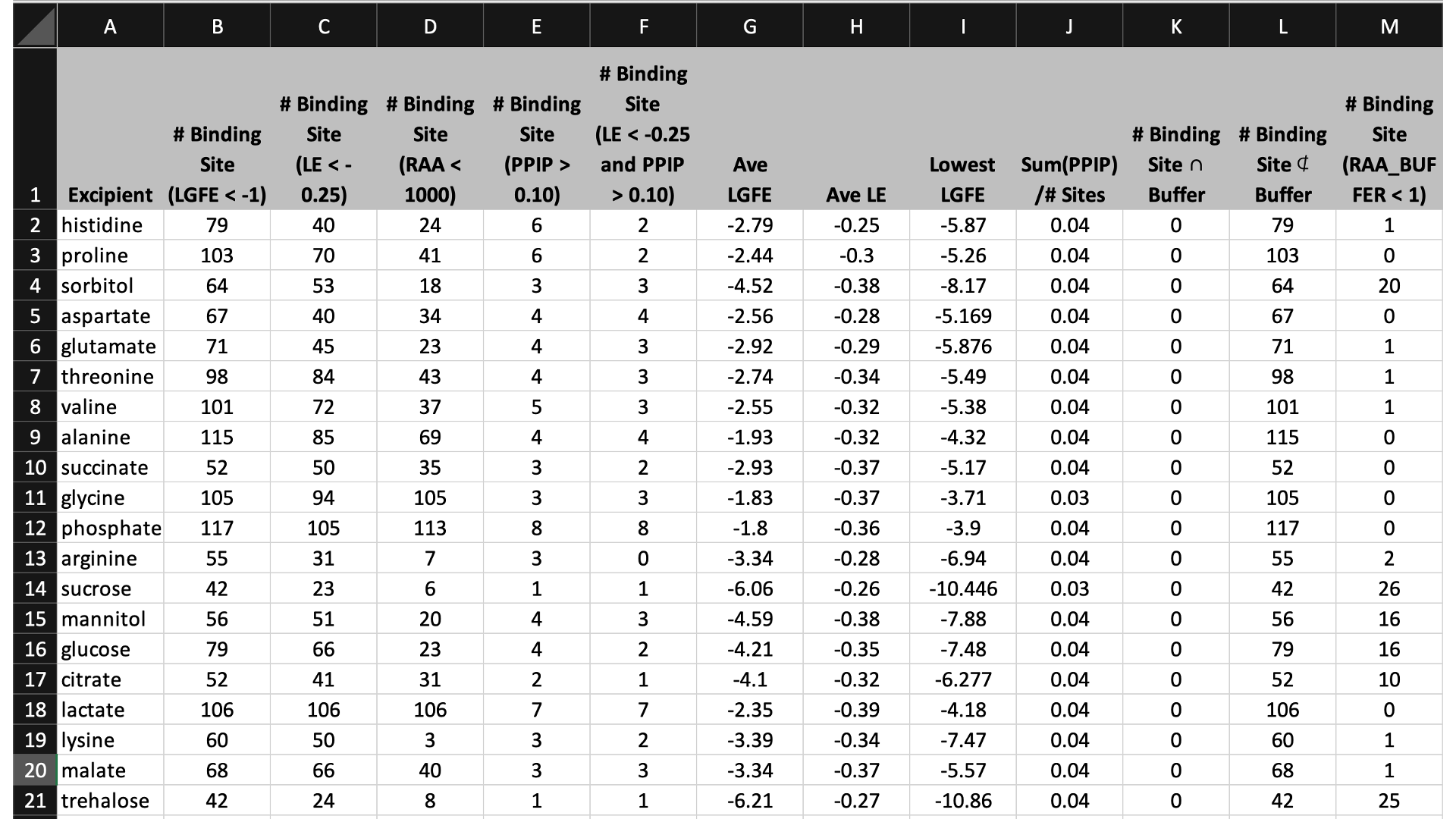
The contents of the columns are:
A: The excipient.
B: The number of binding sites where the excipient binds with an Ligand Grid Free Energy (LGFE) < -1 kcal/mol. LGFE approximates the binding affinity.
C: The number of binding sites where the excipient Ligand Efficiency (LE) < -0.25 kcal/mol. LE provides a metric of the binding affinity normalized for molecular size. LE = LGFE / N_heavy_atom, where N_heavy_atom is the number of non-hydrogen atoms in the excipient.
D: The number of binding sites found with a Relative Affinity Analysis metric (RAA) < 1000. RAA indicates the number of “strong” binding sites accessible to each molecule. The RAA is a ratio of dissociation constants (Kd’s), where the numerator is the Kd for the excipient at a given pocket and the denominator is the Kd for the best-scoring (highest affinity) binding pose for that excipient across the entire protein. Kd is computed from LGFE, where LGFE is taken to be the free energy.
E: The number of binding sites with a sum of PPI preference for residues in the binding site (PPIP) > 0.10. A high PPIP value for a binding site suggests that site is more likely to contribute to a PPI.
F: The number of binding sites having both LE < -0.25 kcal/mol and PPIP > 0.10.
G: The average LGFE for the excipient.
H: The average LE for the excipient.
I: The LGFE for the best-scoring (highest affinity) pose of the excipient.
J: Sum(PPIP)/# sites is the sum of the PPIP values for all of the binding sites in column B divided by the value of column B. This gives an average PPIP value computed accross the excipient-favored binding sites.
K: The number of binding sites that overlap with buffer binding sites. If no buffer was specified, this number will be zero. If all excipient binding sites are also capable of binding buffer, this number will be equal to the value in column B.
L: The number of excipient binding sites that are not also buffer binding sites. If no buffer was specified, this number will be equal to the value in column B.
M: The number of binding sites where the excipient has a higher binding affinity (i.e, lower Kd or, equivalently, more negative LGFE) than the buffer at that site. In otherwords, the number of binding sites where this excipient will out-compete buffer for binding. If no buffer was specified, this computation is done relative to a hypotheical buffer with an LGFE of -4 kcal/mol.
$WORKDIR/4_report.$job_id/report_output.xlsx contains fractional occupancy
data for excipient binding sites. Individual sheets or tabs in this file
correspond to separate input formulations. Information includes the excipients
and buffer that bind at each site identified for that formulation along
with selected SILCS metrics associated with the occupancy calculations and
PPI interactions. The top row identifies the buffer and excipients used in
that particular formulation along with their concentrations.
With regard to occupancies,
Kd: dissociation constant, such that LGFE=R*T*ln(Kd)
[L]: concentration of the ligand/excipient, with unit Wt/V (g/mL) % => mM
Occupancy = [L]/([L] + Kd) and has range (0, 1). A high occupancy value (close to 1) means that excipient molecule has a high probability of binding at the site. NOTE: Occupany values relative to buffer are also accessible.
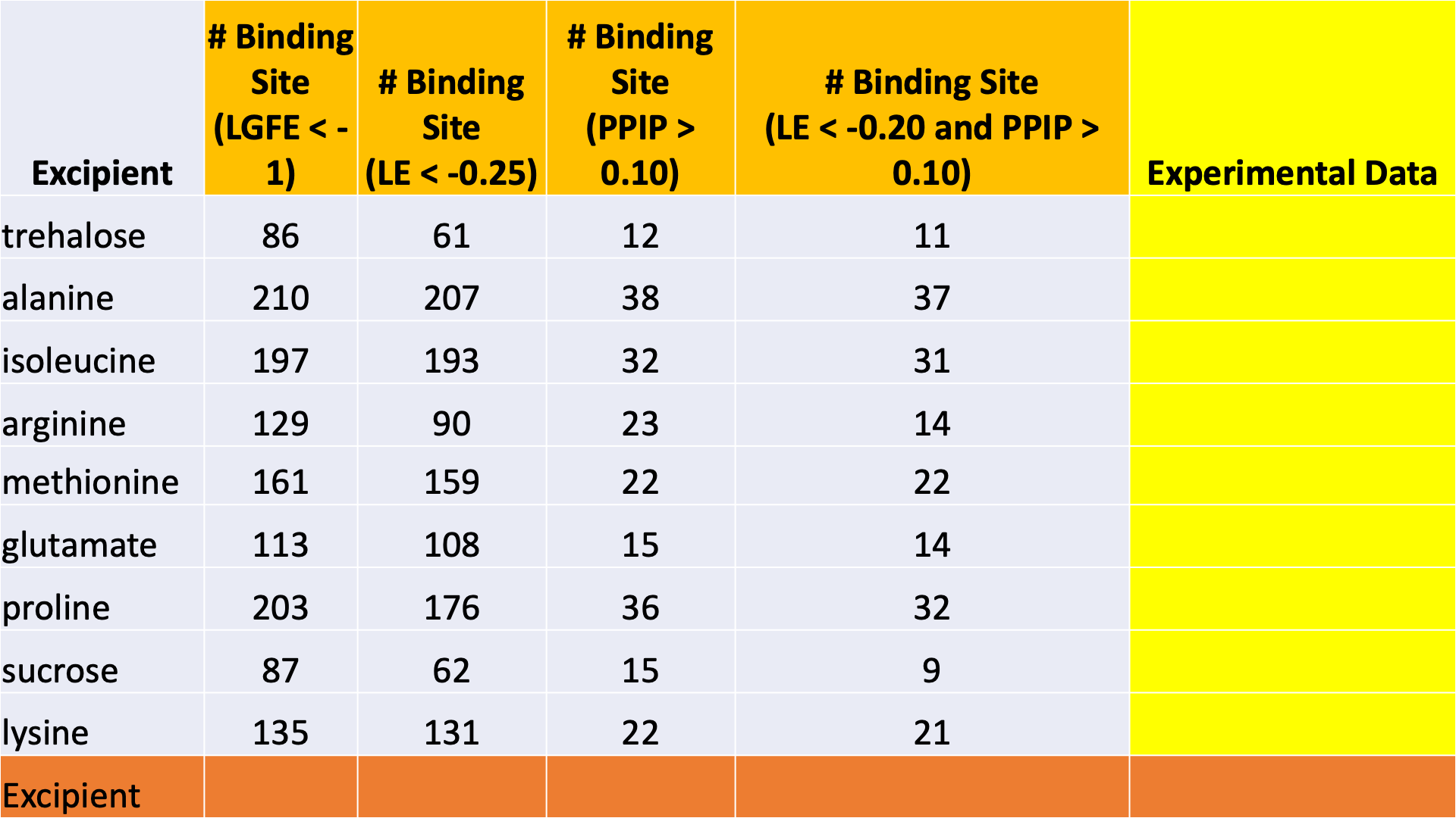
Below is an example of fractional occupancy data. The example metrics assume an occupancy cutoff of 0.8. This and other terms may be varied for reporting.
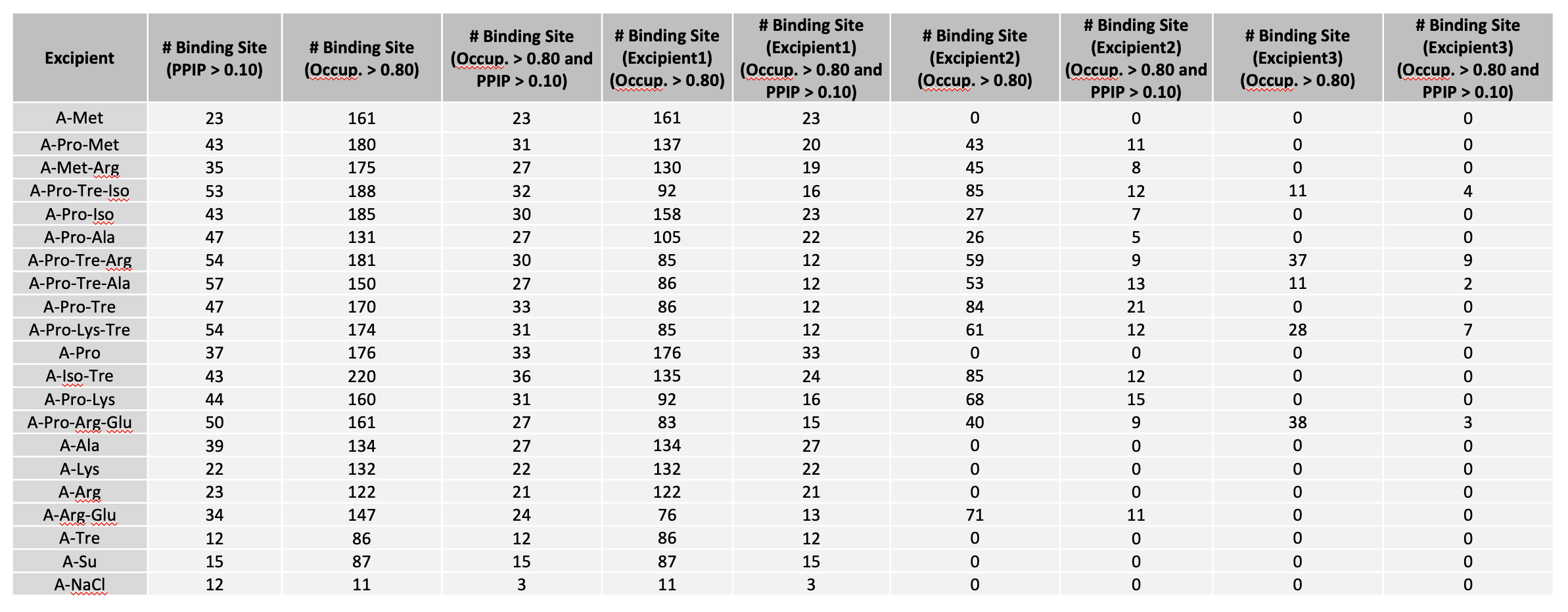
“# Binding Site (Excipient1),(Occup. > 0.80)” suggests the number of excipient binding sites with occupancy > 0.8. If the formulation has multiple excipients, then “excipient1” also represents the excipient with the most binding sites, n comparison with other excipient(s).
“# Binding Site (Excipient2),(Occup. > 0.80)” suggests the number of sites occupied by the excipient with 2nd most binding sites.
“# Binding Site (Excipient3),(Occup. > 0.80)” suggests the number of sites occupied by the excipient with 3rd most binding sites.
“# Binding Site (Excipient1), (Occup. > 0.80 and PPIP > 0.10)” suggests the number of excipient binding sites with high occupancy that coincide with likely PPI. If the formulation has multiple different excipients, then “excipient1” also represents the excipient with the most binding sites, in comparison with other excipient(s).
“# Binding Site (Excipient2),(Occup. > 0.80 and PPIP > 0.10)” suggests the number of second most excipient binding sites with high occupancy that coincide with likely PPI.
“# Binding Site (Excipient3),(Occup. > 0.80 and PPIP > 0.10)” suggests the number of third most excipient binding sites with high occupancy that coincide with likely PPI.
“# Binding Site (Occup. > 0.80)” is the sum of any excipient binding sites with high occupancy. Each binding site with higher occupancy will be counted once.
“# Binding Site (PPIP > 0.1)” suggests the number of all excipient binding sites that coincide with potential PPI.
“# Binding Site (Occup. > 0.80 and PPIP > 0.10)” is the sum of all excipient binding sites with high occupancy that coincide with likely PPI.
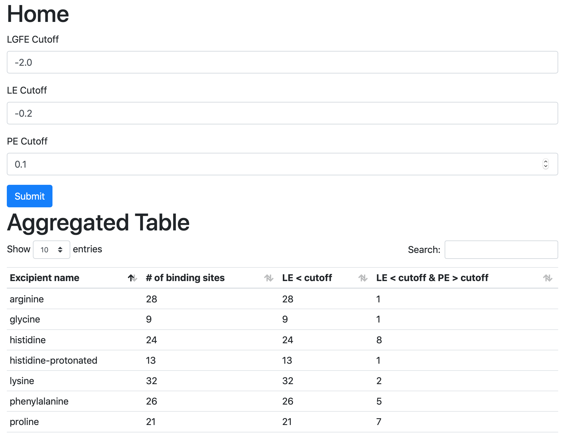
Viewing through a Web Browser
While a spreadsheet application or the SilcsBio GUI is the preferred means to
view .xlsx files, a web view option is available for report_all.xlsx:
cd $WORKDIR/4_report.$job_id/view
sh run.sh
sh run.sh will print out a message like:
* Serving Flask app "main.py" (lazy loading)
* Environment: development
* Debug mode: on
* Running on http://0.0.0.0:5000/ (Press CTRL+C to quit)
* Restarting with stat
* Debugger is active!
* Debugger PIN: 222-574-256
Open a web browser and go to the URL displayed in the output (e.g., http://127.0.0.1:5000 or http://<IP address>:5000).
If you are running the web view from a remote server and if the server is behind a firewall, you may not able to directly access the web view. In this case, you can use a method called SSH port forwarding. This uses an SSH connection to the remote server to access the web view securely.
If you are using Linux, MacOS, or Linux subsystem on Windows as your desktop:
Open a terminal;
SSH to the remote server using the following example SSH command in the terminal;
ssh -L 5000:localhost:5000 username@servernameOpen a tab in the web browser, and navigate to
localhost:5000.
If you are using Windows as your desktop and the PuTTY application for SSH access:
Open PuTTY
Select “Session”, and
Type in the target host name and port (default: 22);
Choose SSH as the connection type (default);
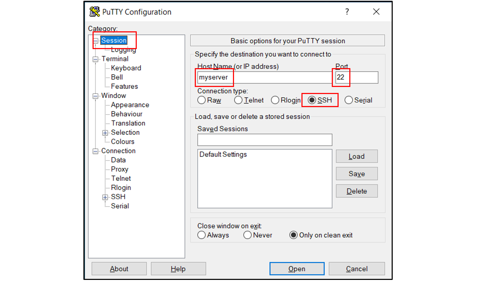
Select “Connection -> Data”, and
Type in your username as the auto-login username
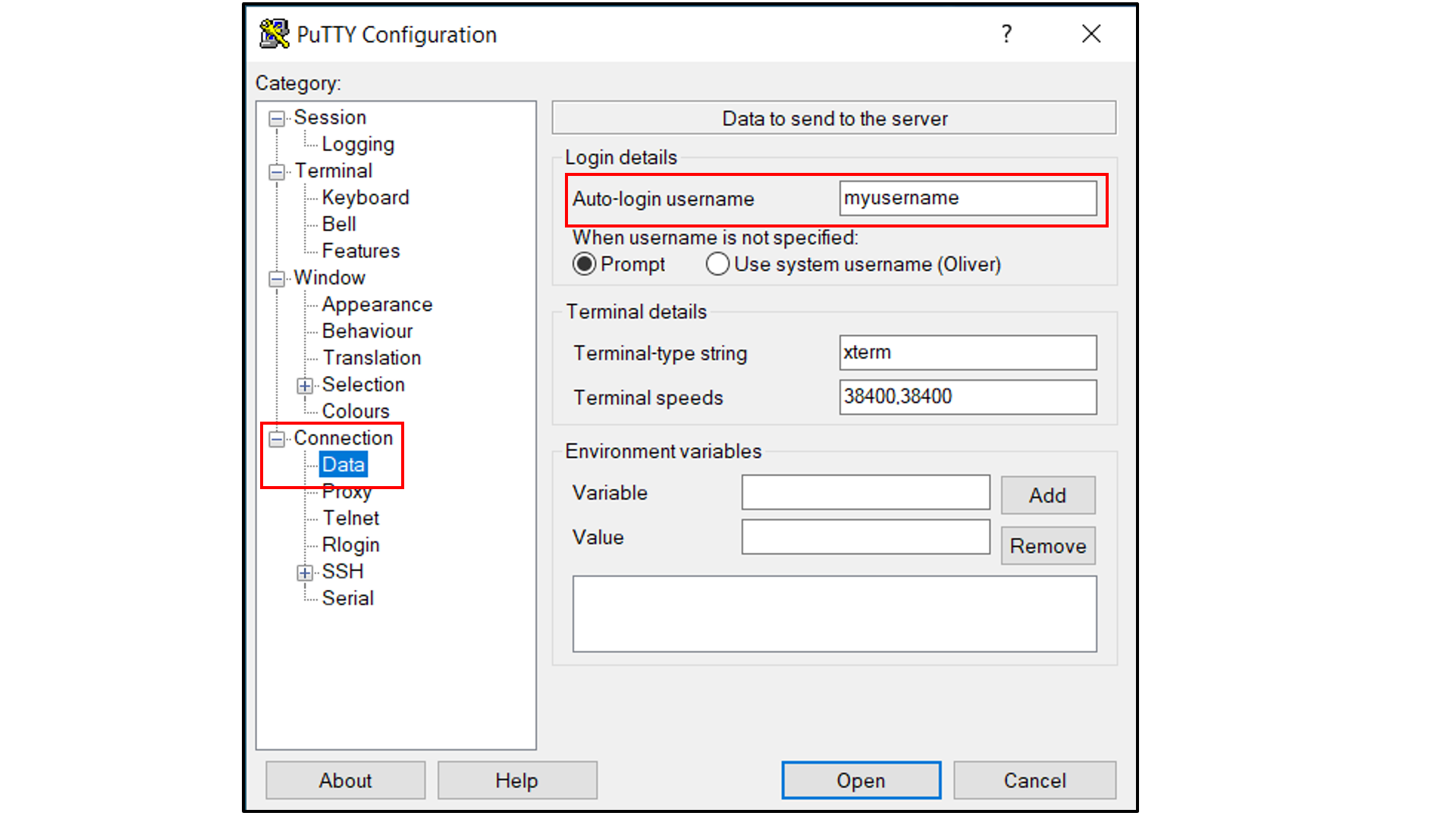
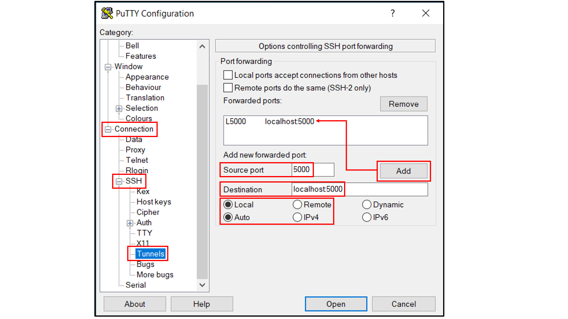
Select “Connection -> SSH -> Tunnels”, and
In “Source port”, type in
5000;In “Destination”, type in
localhost:5000;Click the “Add” button on the right side of “Source port” box;
Turn on the Local and Auto radio buttions (default) below the “Destination” box;
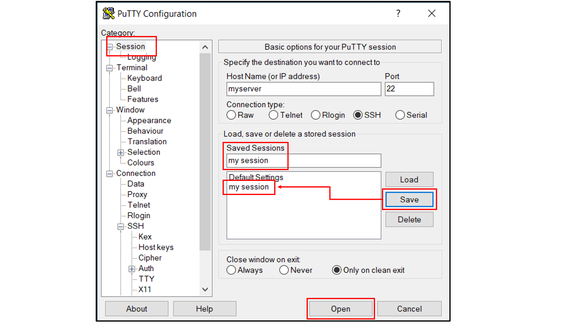
Select “Session”, and
Choose a name for the session;
Click the “Save” button to save the session with all your parameters;
Click “Open” to open a terminal to connect to your remote server.
Open a tab in the web browser, and navigate to
localhost:5000.
Data Interpretation
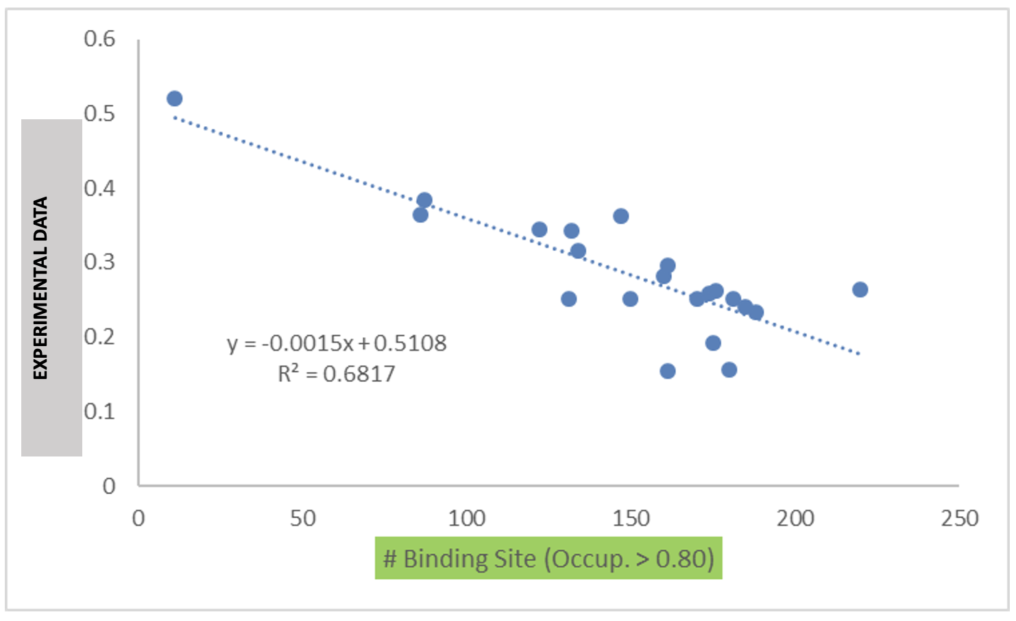
The data output from Step 4 can help connect experimental observables to the molecular details of protein-excipient interactions. In doing so, these simulation data can help both rationalize known trends for existing data on excipients and suggest the choice of new excipients for additional testing. With regard to the former, the most straightforward approach is to compare available experimental data to the Step 4 output and note correlations:
Please see [2] for a real-world example.
Below is an example of blinded data from a collaboration case study that
demonstrates the utility of the binding site occupancy metrics computed
by SILCS-Biologics and available in report_output.xlsx:
Visualizing SILCS FragMaps and SILCS-PPI Results
Tip
If you ran your SILCS-Biologics workflow using the SilcsBio GUI, SILCS FragMaps and SILCS-PPI results visualization will be available to you directly in the SilcsBio GUI upon successful completion of your SILCS-Biologics job. Please refer to SILCS-Biologics Using the GUI for more information.
SILCS FragMaps generated during Step 1 of the SILCS-Biologics workflow can
be easily visualized using your choice of MOE, PyMol, or VMD molecular
graphics software packages. FragMaps will be located in
$WORKDIR/1_fragmap.$job_id/fab/silcs_fragmaps_fab. Please see
Visualizing SILCS FragMaps for detailed instructions.
SILCS-Biologics Step 2 SILCS-PPI results can also be viewed using
molecular graphics software. For the purposes of SILCS-PPI, one protein
is considered the “receptor” and the other the “ligand”. In the current
use case with only one input protein domain, prot1=fab.pdb,
fab.pdb data are used for both the “receptor” and the “ligand”. For
the purpose of SILCS-PPI, the ligand protein is docked to the receptor
protein by comprehensively sampling locations and orientations of the
ligand protein relative to the receptor protein. The relative locations
and orientations are scored based on the overlap of the ligand
functional groups and the receptor protein SILCS FragMaps (computed in
Step 1). The docked poses of the ligand are then clustered as part of
SILCS-PPI.
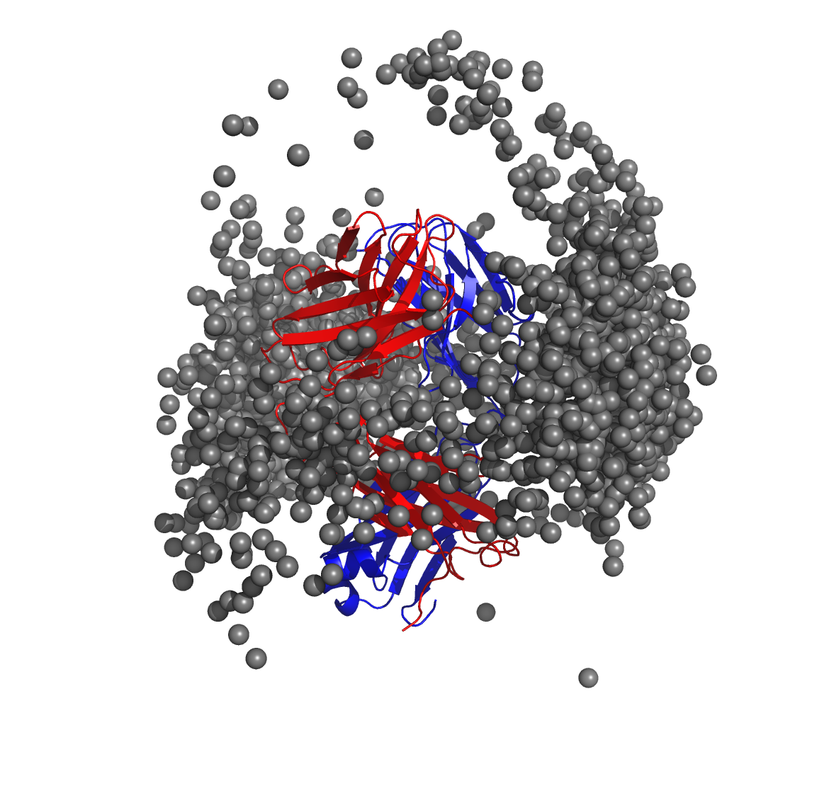
The $WORKDIR/2_ppi.$job_id/fab_fab/3_ppi/receptor_clusters.pdb file
contains the receptor protein structure and the cluster centroids. The
cluster centroids in this file all have the same chain name, Z.
Below is a molecular graphics image of receptor_clusters.pdb, with
the receptor protein shown as ribbons and the cluster centroids as
spheres. The CDR loops of the Fab are pointing to the top of the image,
heavy chain amino acids are in red, light chain amino acids are in blue,
and cluster centroids are in gray.
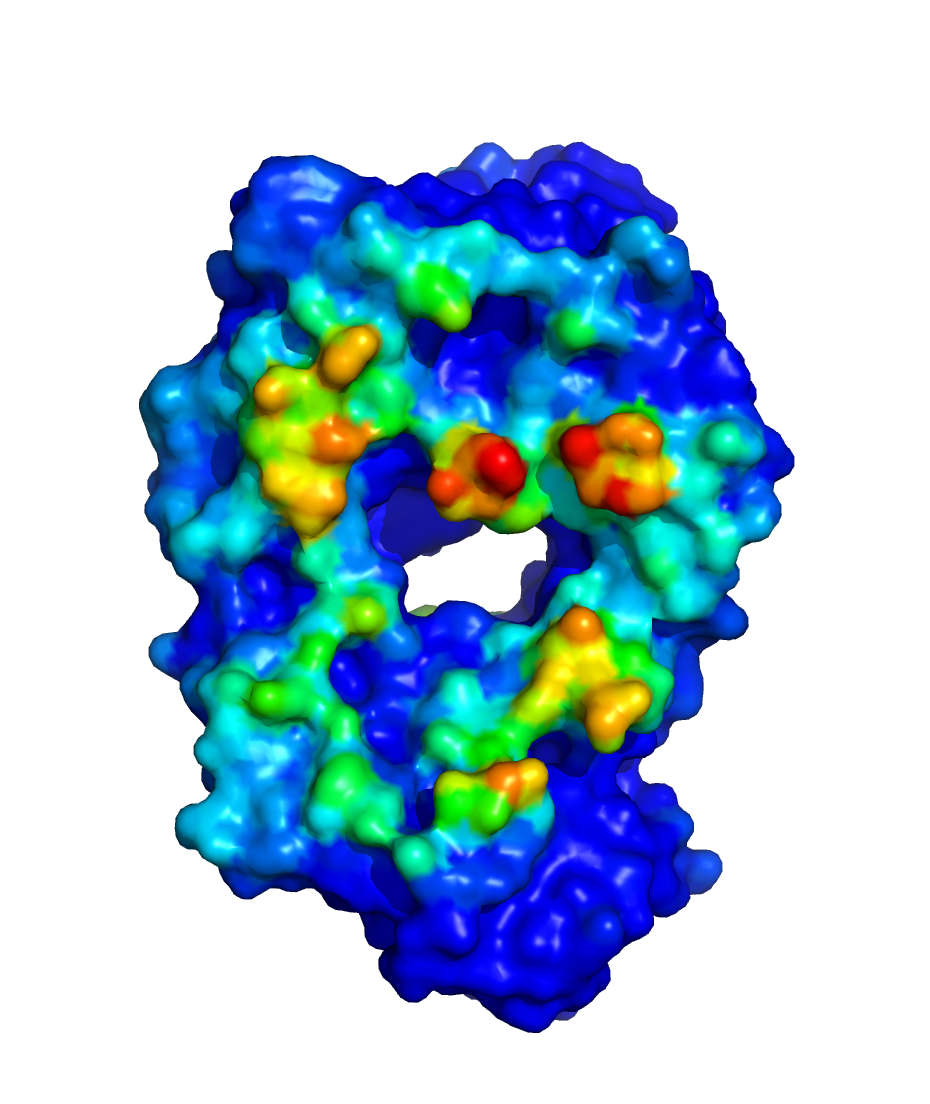
$WORKDIR/2_ppi.$job_id/fab_fab/3_ppi/receptor_surf_contact.pdb
contains PPI propensity values mapped onto the receptor protein and
recorded in the B-factor column, which provides an easy way to visualize
which residues are most at risk for contributing to PPI, and, therefore,
to aggregation of the biologic in its native (folded) state: