Graphical User Interface (GUI) Quickstart
This chapter provides a step-by-step introduction on how to use the SilcsBio Graphical User Interface (GUI).
SilcsBio GUI Suite Selection
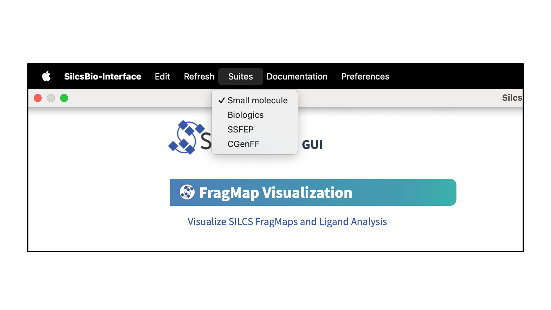
The SilcsBio GUI provides convenient access to cutting-edge SILCS and CGenFF technologies for computer-aided drug discovery. Currently, four suites are available through the SilcsBio GUI:
Small Molecule Suite
Biologics Suite
SSFEP Suite
CGenFF Suite
Upon opening the SilcsBio GUI, the user will directly enter the SILCS-Small Molecule Suite. To access different suites, select the desired suite from the menu bar.
Additional information on the capabilities of each suite are overviewed in the current chapter as well as detailed in the following chapters of this documentation.
Remote Server Setup
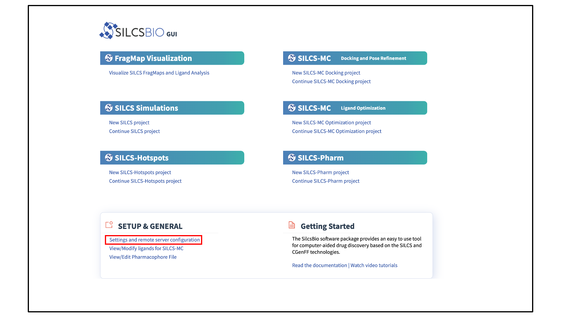
The SilcsBio GUI is designed to work with the server installation of the SilcsBio software. Launch the GUI and select Settings and remote server configuration.
Within the “Settings and remote server configuration” page, select Server and enter the remote server information, such as Server Address (IP address), Username, and an SSH key to the server. If you do not have an SSH key to the server, leave it blank. The GUI will ask you the password to the remote server instead. Select the “Make Default Server” checkbox if you would like to set this server as your default server. This server will be selected as a default in other parts of the GUI.
You will also need to enter SILCSBIODIR and GMXDIR file path values.
These should match the values on your server. You may use the
“Extra setup” field to pass additional commands to the server, such as
exporting environment variables or loading modulefiles.
Note
The SilcsBio GUI will enter a reset environment on the remote server. Thus, you need to manually add all necessary packages (e.g., python) in the PATH.
You may use the “Project Directory” field to define the directory on your server where server job input files will be created and server job outputs stored. Typical SILCS simulations produce output files in excess of 100 GB, so please select a project directory file folder with appropriate storage capacity. The “SILCS NUMSYS” field determines how many SILCS jobs are launched for creating FragMaps. Set this to an even integer; we recommend “10” to maximize convergence or “8” to minimize resource use.
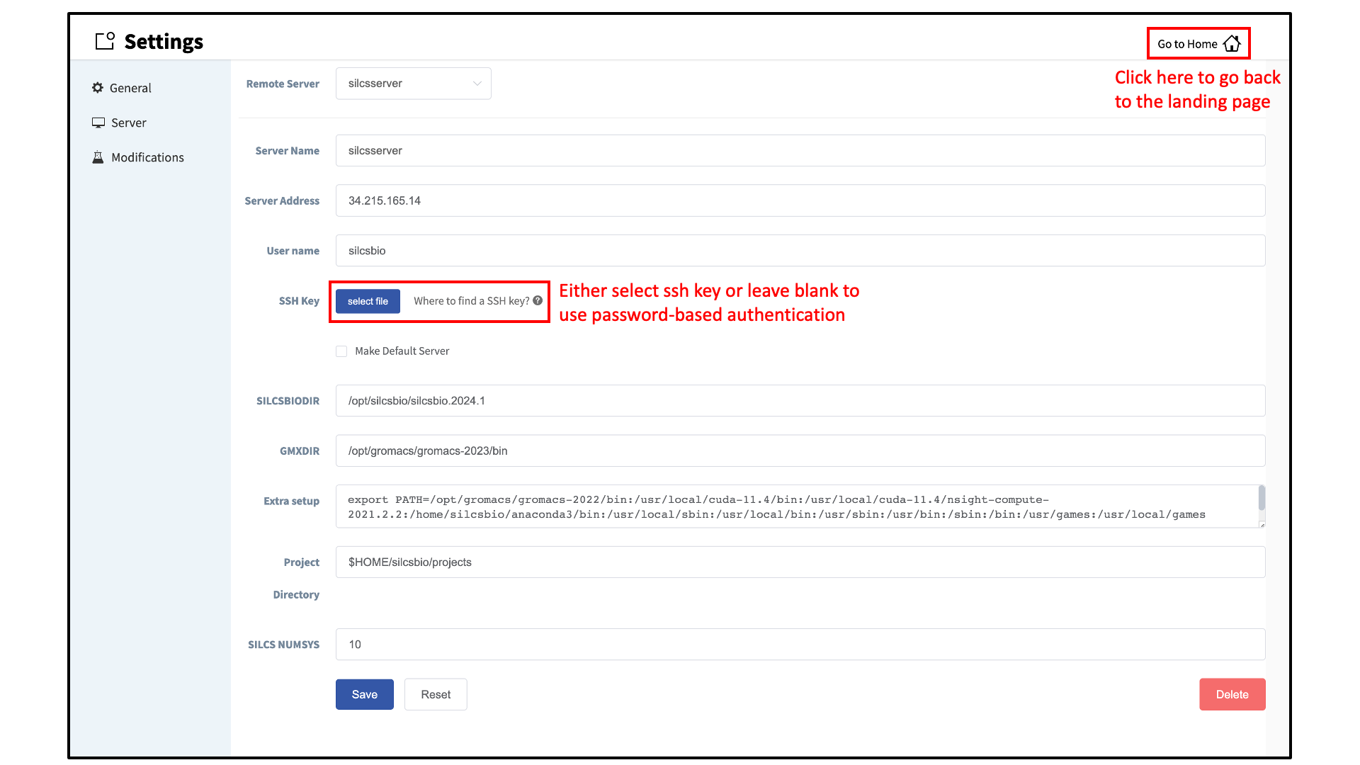
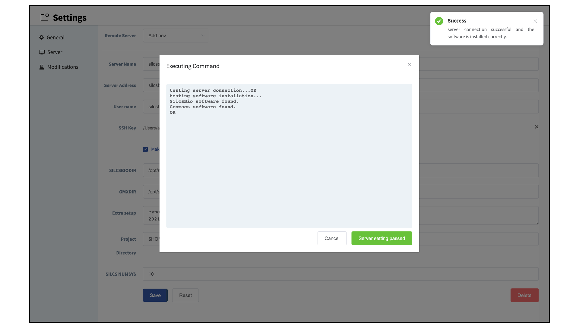
Once all information is entered, click the “Save” button. The GUI will save your entries and confirm that you have a working connection to the server.
Please contact support@silcsbio.com if you need additional assistance.
File and Directory Selection
To run the SilcsBio software, you will need to provide protein and/or ligand input files. The SilcsBio GUI has a standardized user interface that allows you to choose these input files from either the computer on which you are running the GUI or from a remote server you have previously configured. Steps to do this, illustrated in the below figures, are as follows:
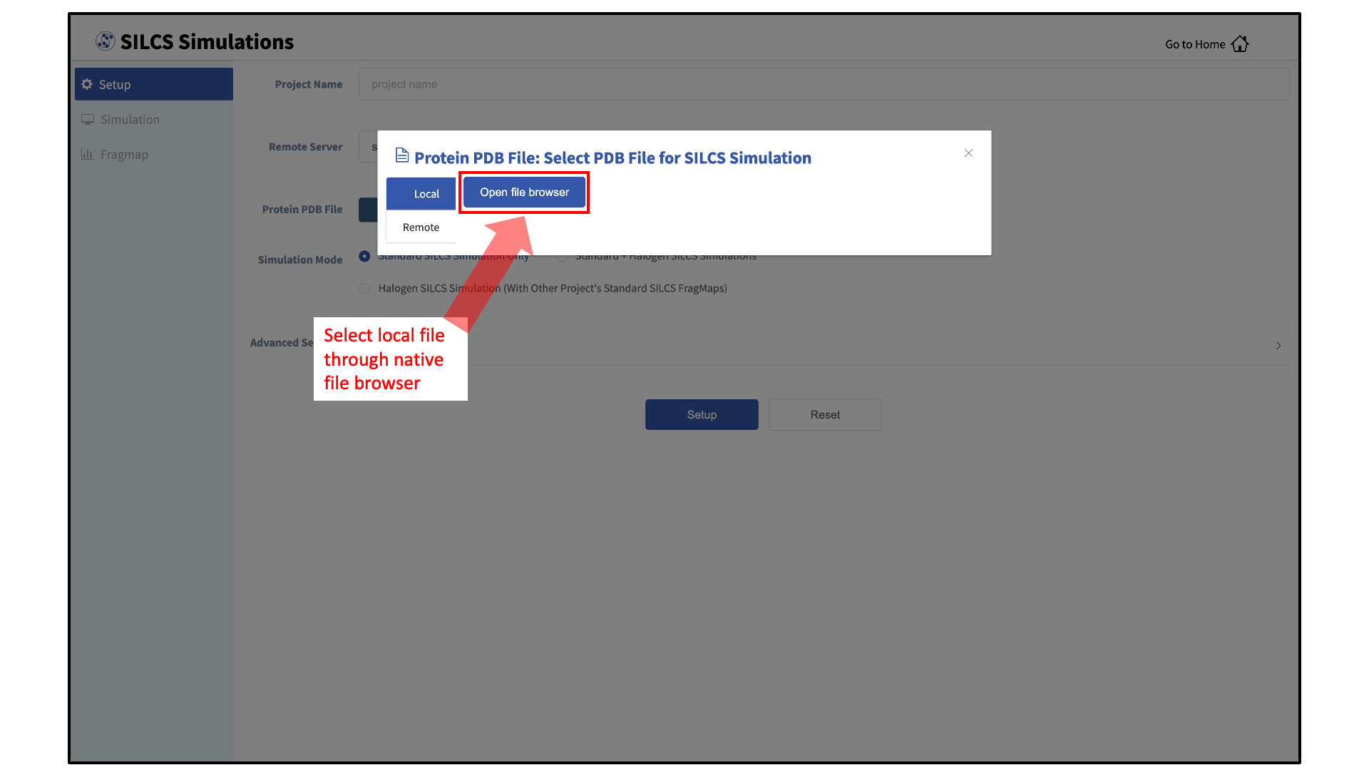
Choose the server on which is the physical location of the input file is located. If you would like to load a file located on the computer on which you are running the GUI, click Local; otherwise, click Remote and select the remote server name of a server you have previously configured through the Remote Server Setup process.
If the file is located on the local computer, click Open file browser. This will open your local computer’s native file browser. Select your file following the conventions of your local computer.
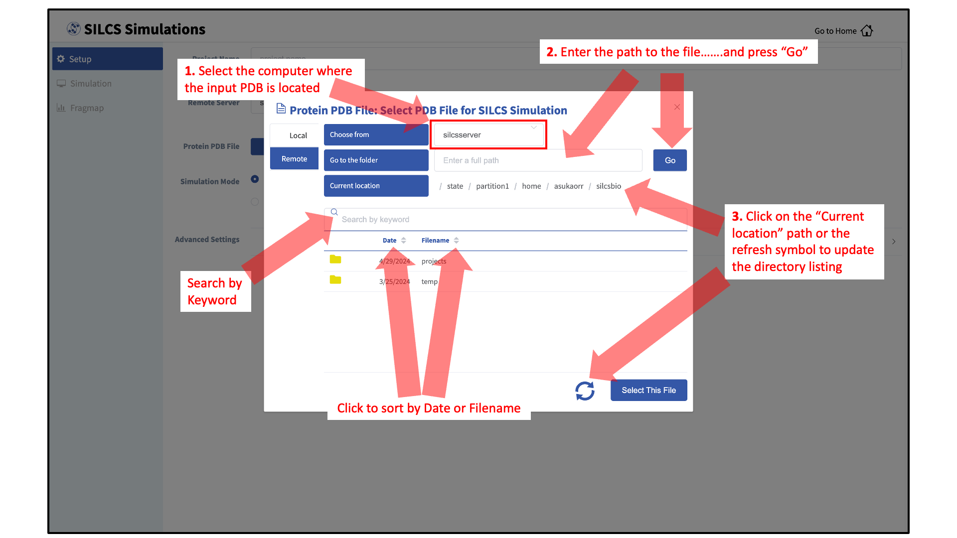
Otherwise, if the file is located on a remote server, type in the folder where the file is located using the “Go to the folder” field and then click the associated Go button. This will update the “Current location” to this folder. Click on the last portion of the “Current location” path (e.g. “silcsbio” in “/state/partition1/home/asukaorr/silsbio” in the below example) to update the directory listing located under that path. If you click on any other portion of the “Current location” path, you will be taken to that folder. Double clicking on a folder in the directory listing will move you into that folder. In the directory listing, click on a file to highlight it and click the Select This File button at the bottom to finish your file selection.
Follow a similar process to select a directory for those tasks requiring directory selection.
Tip
For those tasks needing FragMaps as inputs, “FragMap Location” needs
to be a directory. The SilcsBio GUI
assumes a directory path of the form <basename>/maps/. Select
<basename> for your “FragMap Location”. The GUI will automatically
look for the maps/ subdirectory and load FragMaps from that
subdirectory. It will also automatically load the protein pdb file if
one is located in the <basename> directory. It may take
a few seconds for the GUI to download your input FragMaps if they are
not on localhost.
SILCS-Small Molecule Suite Quickstart
When the SilcsBio GUI is opened, the user will directly enter the Small Molecule Suite. The Home page of the Small Molecule Suite features a number of SILCS technologies.
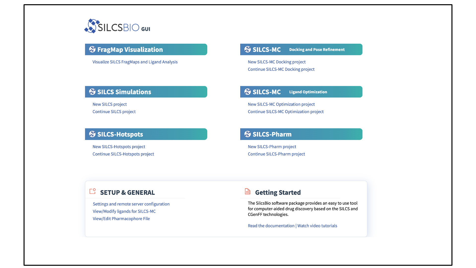
The SILCS technologies can be combined to follow a logical order for computer-aided drug discovery/design:
Target proteins are characterized by SILCS FragMaps using SILCS Simulations.
Potential binding sites are identified using SILCS-Hotspots.
Pharmacophore models are built at identified binding sites using SILCS-Pharmacophore.
Potential drugs are docked and evaluated with SILCS-MC Docking and Pose Refinement.
Lead compounds are modified and optimized using SILCS-MC Ligand Optimization.
All SILCS technologies revolve around FragMaps generated from SILCS simulations. A quickstart to visualize SILCS FragMaps (SILCS FragMap Visualization Quickstart) and to perform the SILCS simulations needed to generate SILCS FragMaps is provided in this chapter (SILCS Simulations Using the GUI) with additional details on SILCS simulations provided in SILCS Simulations. Information on the background and usage of SILCS-Hotspots, SILCS-Pharmacophore, SILCS-MC Docking and Pose Refinement, and SILCS-MC Ligand Optimization are provided in SILCS-Hotspots, SILCS-Pharm, SILCS-MC: Docking and Pose Refinement, and SILCS-MC: Ligand Optimization, respectively.
The Small Molecule Suite also provides convenient access to general tools under SETUP & GENERAL at the bottom of the page:
For additional information on these tools, please click on their links.
SILCS FragMap Visualization Quickstart
The SilcsBio GUI provides a convenient platform to visualize FragMaps, as described below. FragMaps can also be visualized using MOE, PyMOL, and VMD as described in Visualizing SILCS FragMaps. The following instructions outlines the features in the SilcsBio GUI tool for visualizeing FragMaps:
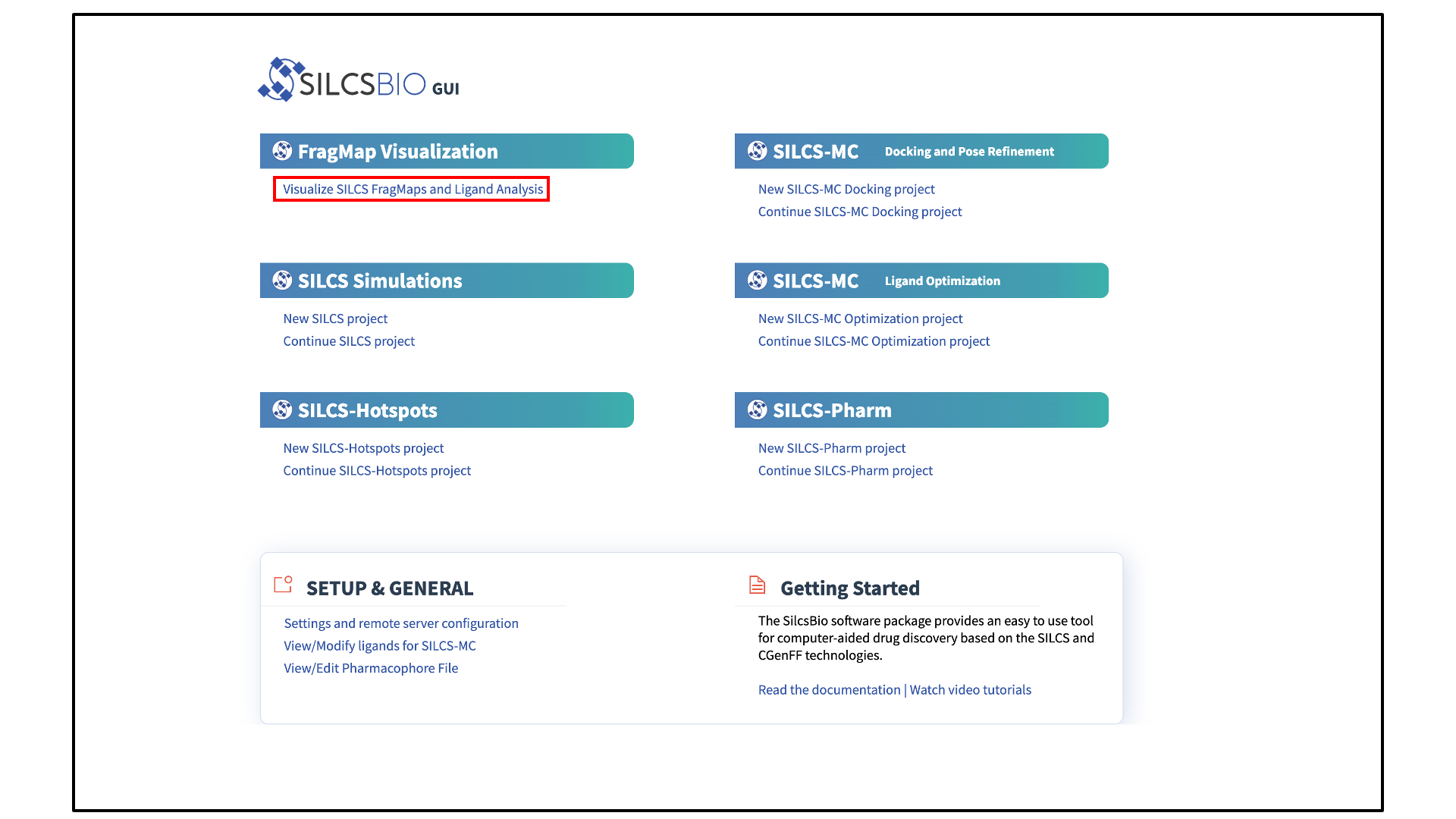
Open the FragMaps visualization tool:
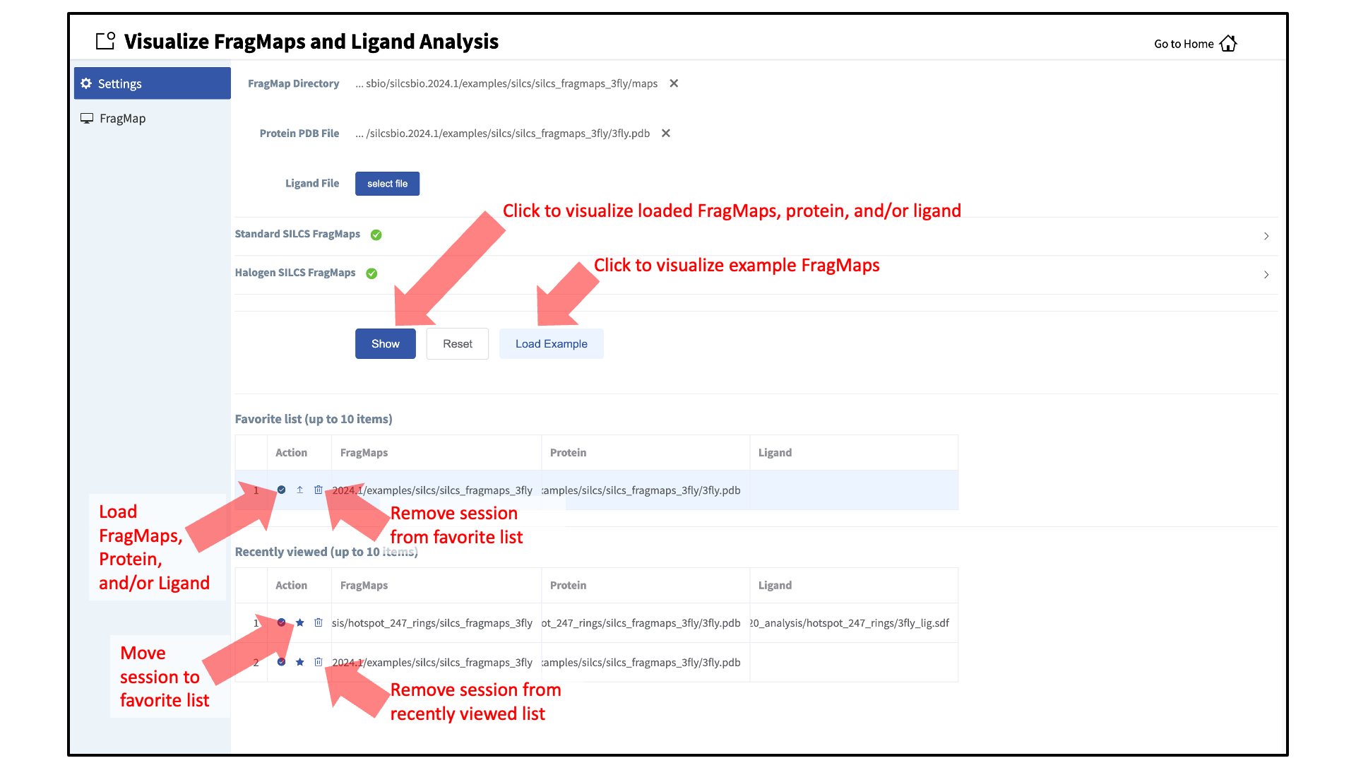
The FragMaps visualization tool can be accessed by clicking Visualize SILCS FragMaps and Ligand Analysis at the bottom of the Home page of the SilcsBio GUI:
If you are loading SILCS FragMaps from the Home page, you will be asked to select your FragMap directory (see File and Directory Selection). This directory has a standard name,
silcs_fragmaps_<protein PDB>, where<protein PDB>is the name of the input PDB file. This directory was created on the server where you ran the SILCS jobs either when you clicked the “Generate FragMap” button or when you ran the${SILCSBIODIR}/silcs/2c_fragmap prot=<protein PDB>command.In the case the SilcsBio GUI was used to run the SILCS simulations (see SILCS Simulations Using the GUI), once the simulations are complete, the GUI will prompt you to “Generate FragMap” and automatically create FragMaps from the SILCS simulations, download them onto the local computer, and load them, along with the input PDB file, for visualization.
Alternatively, previously viewed visualization sessions may also be loaded by clicking on the checkmark next to the desired session under “Action”. The ten most recently viewed visualization sessions will be listed under “Recently viewed”. Frequently viewed sessions can be saved under the “Favorite list” by clicking on the star icon next to the session under “Action”.
Note
In addition to the FragMaps, the
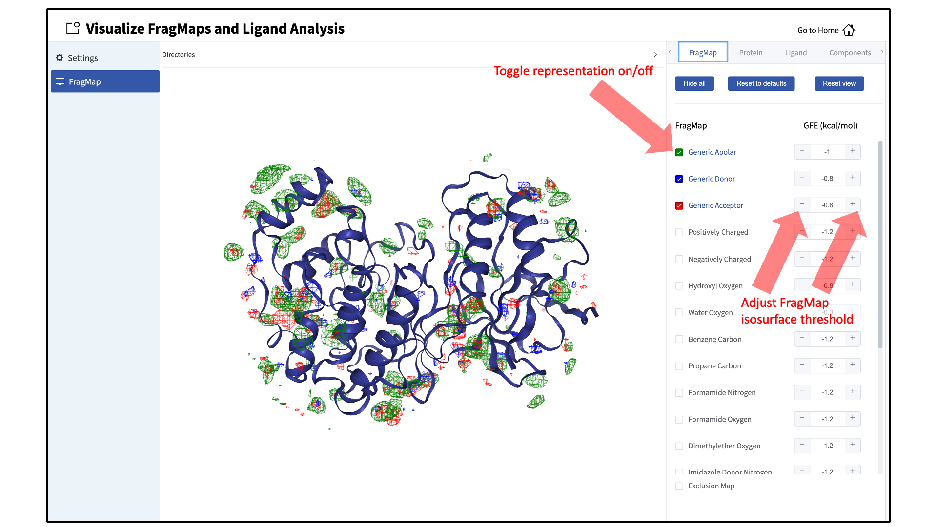
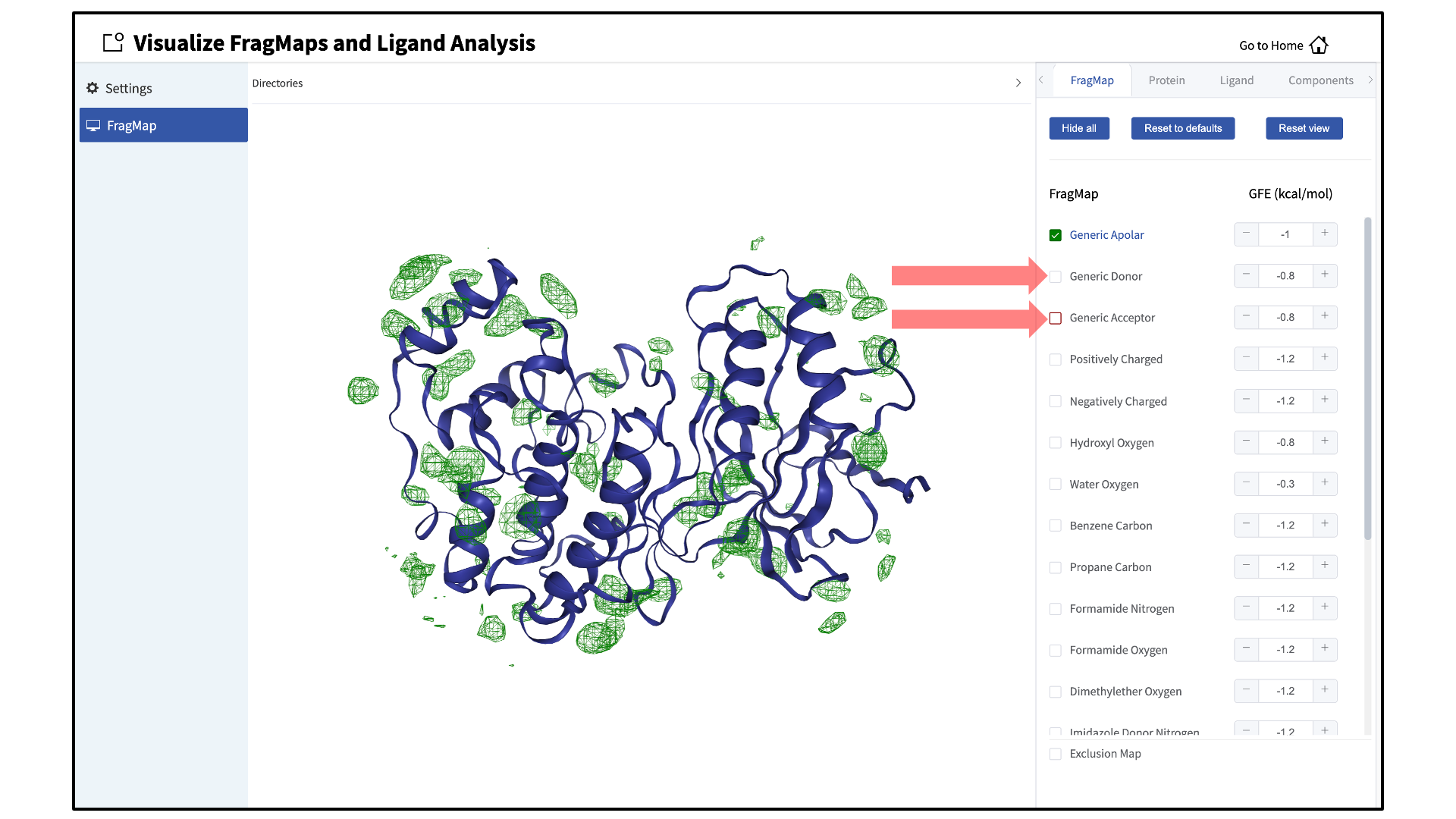
silcs_fragmaps_<protein PDB>directory contains the PDB file used to run the SILCS simulations. The SilcsBio GUI will automatically detect and load this PDB file. Additionally, if you have run Halogen SILCS, this directory will also contain the Halogen SILCS FragMaps, which will be automatically detected and loaded by the GUI.Toggle FragMap and protein representations on/off:
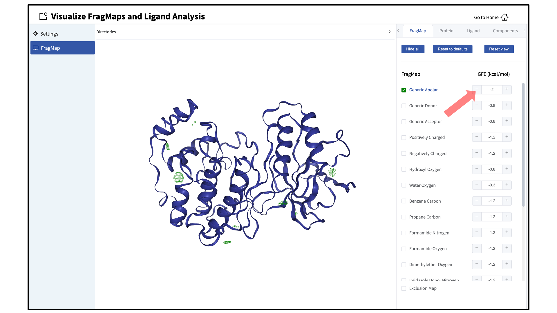
Specific FragMaps can be hidden or shown by toggling the representations on or off. The FragMap isosurface thresholds can also be adjusted to specific GFE values. The input protein may also be shown in surface and cartoon representation or hidden by toggling the protein representations on or off. Additional details on what each FragMap represents can be found in Visualizing SILCS FragMaps.
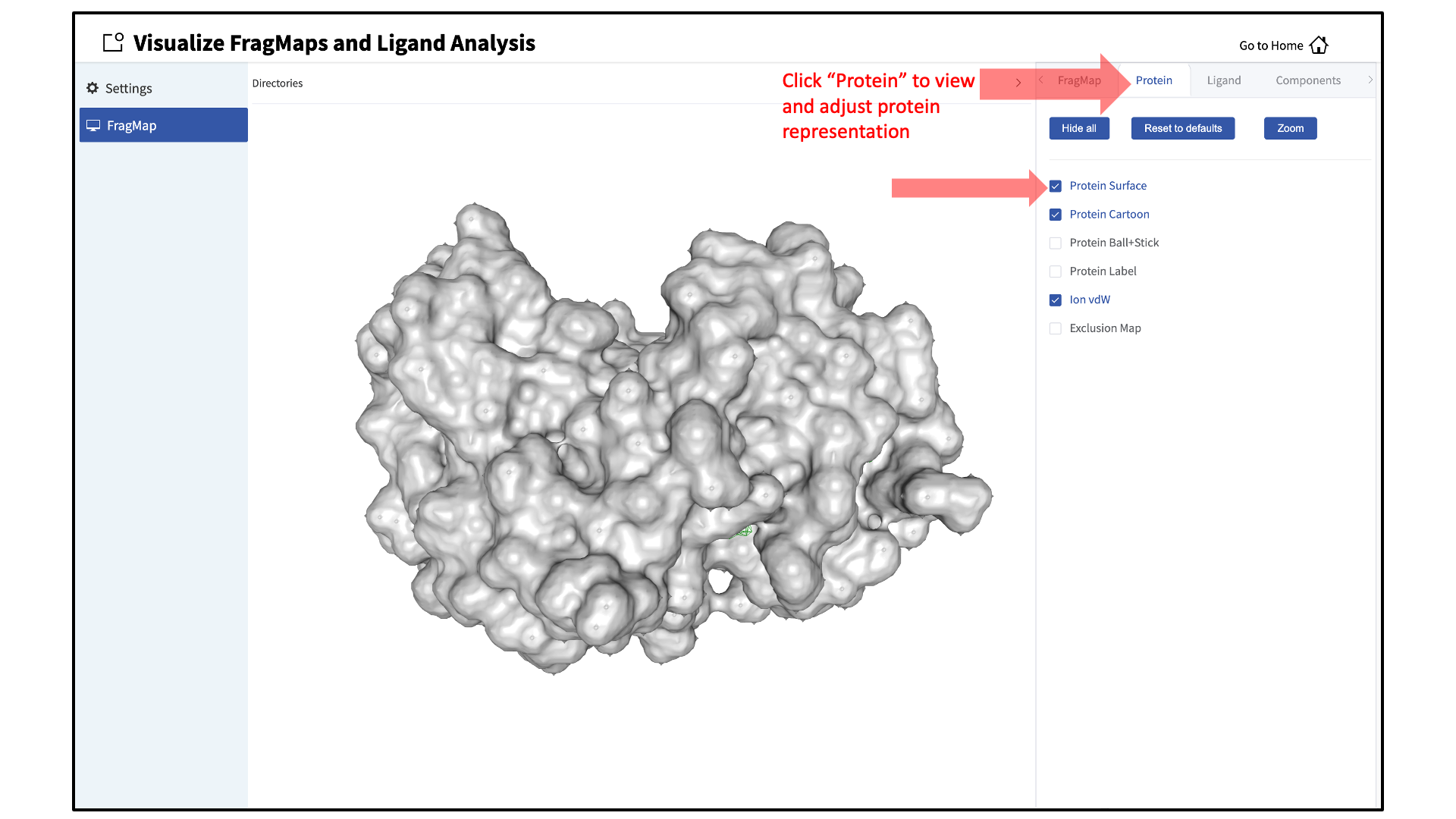
Adjust protein representation:
By default, the protein will be shown in cartoon representation. The representation of the protein can be adjusted by clicking the “Protein” tab of the sidebar menu and toggling on or off the desired protein representations. The default protein representation can be restored by clicking on the Reset to defaults button.
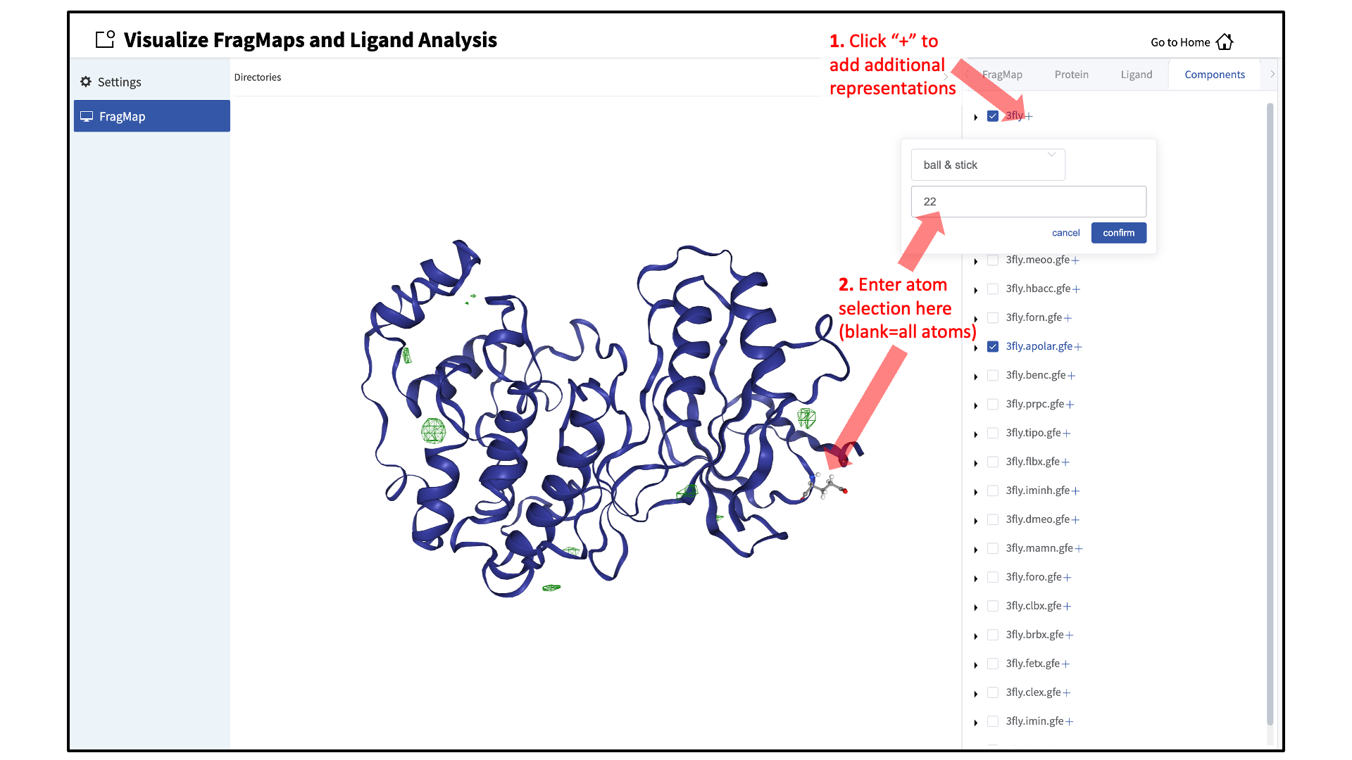
When adding an additional representation, the default is to apply it to all atoms. To apply a representation to a specific set of atoms, click on the “Components” tab of the sidebar menu, click on the “+” adjacent to the protein structure name, and type the atom selection in the blank box above the “cancel” and “confirm” buttons. The selection syntax is the same as for the NGL molecular structure viewer (see Atom Selection in the SilcsBio GUI).
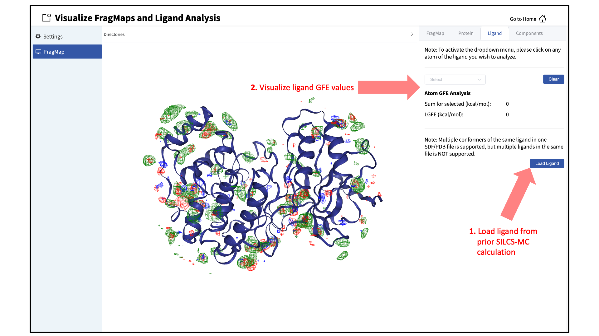
Load ligands for visualization:
It is also possible to load ligands for visualization. If the ligand file was the output of a SILCS-MC calculation, GFE values for the ligand atoms will be embedded within that file. These values can be visualized and their sum automatically computed by first loading the ligand file, and then using the “Ligand” tab as detailed at the end of the section SILCS-MC Ligand Optimization Using the SilcsBio GUI.
SILCS Simulations Using the GUI
To begin a new SILCS project, follow these steps:
Begin a new SILCS project:
Select New SILCS project from the Home page.
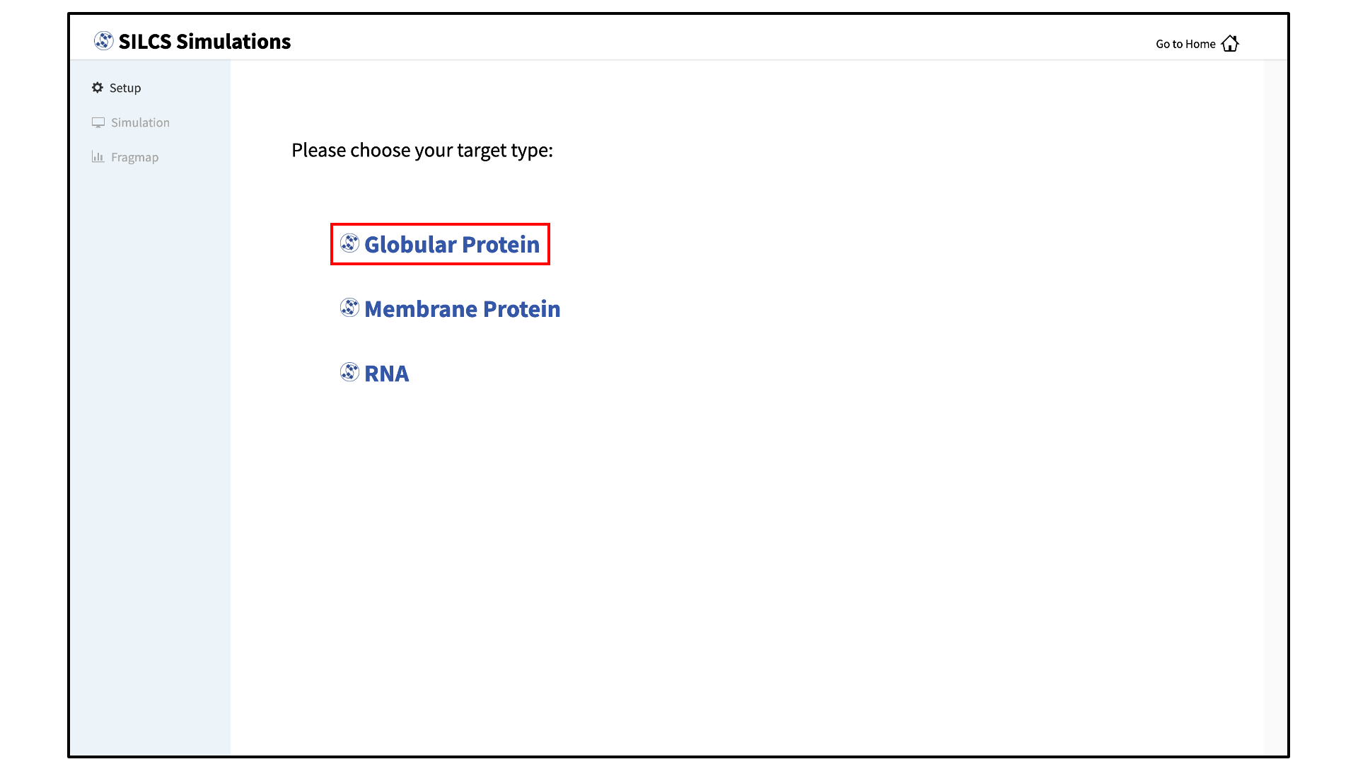
Select the macromolecule target type:
Click on the desired macromolecule type (Globular Protein, Membrane Protein, or RNA). For the purposes of this GUI quickstart, the following instructions are focused on running standard SILCS simulations for Globular Protein target types. For additional details on SILCS for Membrane Protein, or RNA target type, please see SILCS Simulations.
Enter a project name, select the remote server, and upload input files:
Enter a project name and select the remote server where the SILCS jobs will run. Input and output files from the SILCS jobs will be stored on this server based on your choice of “Project Directory” during the Remote Server Setup process.
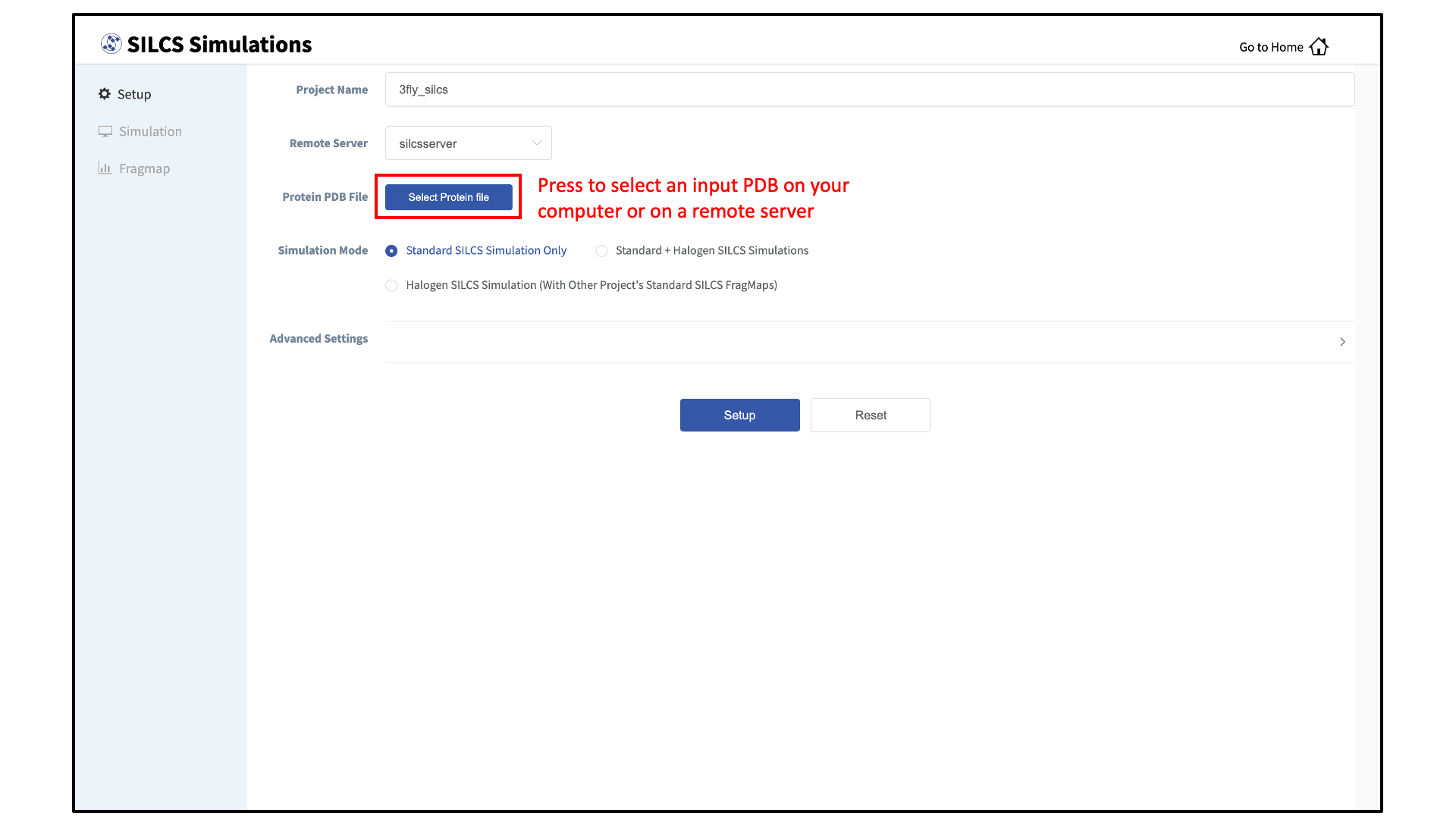
Next, select a protein PDB file. As described in File and Directory Selection, choose a file from your local computer (“localhost”) or from any server you had configured through the Remote Server Setup process. We recommend cleaning your input PDB file before use, incuding keeping only those protein chains that are necessary for the simulation, removing all unnecessary ligands, renaming non-standard residues, filling in missing atomic positions, and, if desired, modeling in missing loops.
If the GUI detects missing non-hydrogen atoms, non-standard residue names, or non-contiguous residue numbering, it will inform the user and provide a button labeled “Fix?”. If this button is clicked, a new PDB file with these problems fixed and with the suffix
_fixedadded to the PDB file base name will be created and used. The SilcsBio GUI will not model residues that are completely missing from the PDB or loops.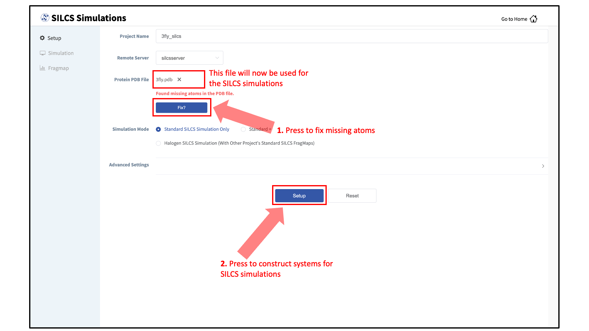
Set up SILCS simulations:
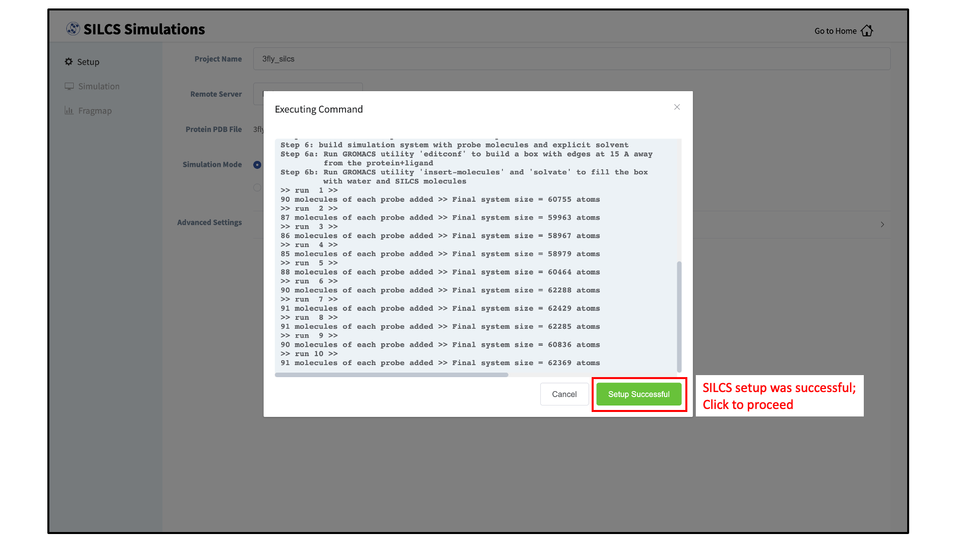
Press the “Setup” button at the bottom of the page. The GUI will contact the remote server and perform the SILCS GCMC/MD setup process. During setup, the program automatically performs several steps: building the topology of the simulation system, creating metal-protein bonds if metal ions are found, rotating side chain orientations to enhance sampling, and putting probe molecules around the protein. To complete the entire process may take up to 10 minutes depending on the system size. A green “Setup Successful” button will appear once the process has successfully completed. Press this button to go to the next step.
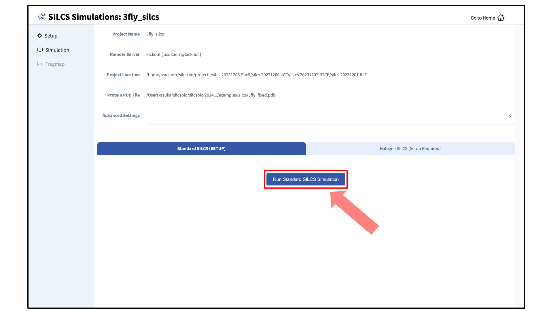
Launch SILCS simulations:
Your SILCS GCMC/MD simulation can now be started by clicking the “Run SILCS Simulation” button. Before running, you may wish to double check that you have chosen the desired file folder on the remote server and that it has 100+ GB of storage space.
Compute jobs will be submitted to the queueing system on the server.
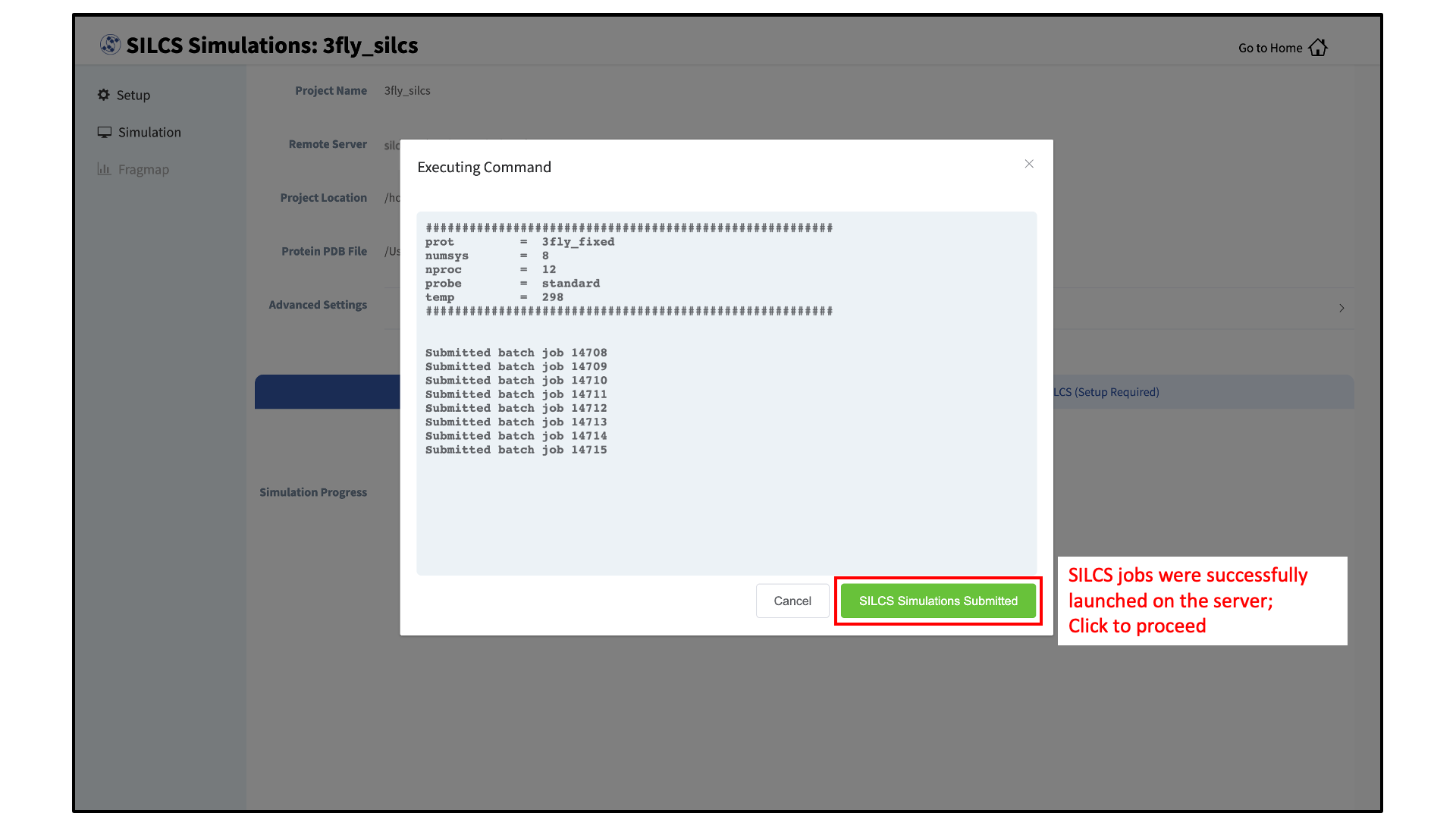
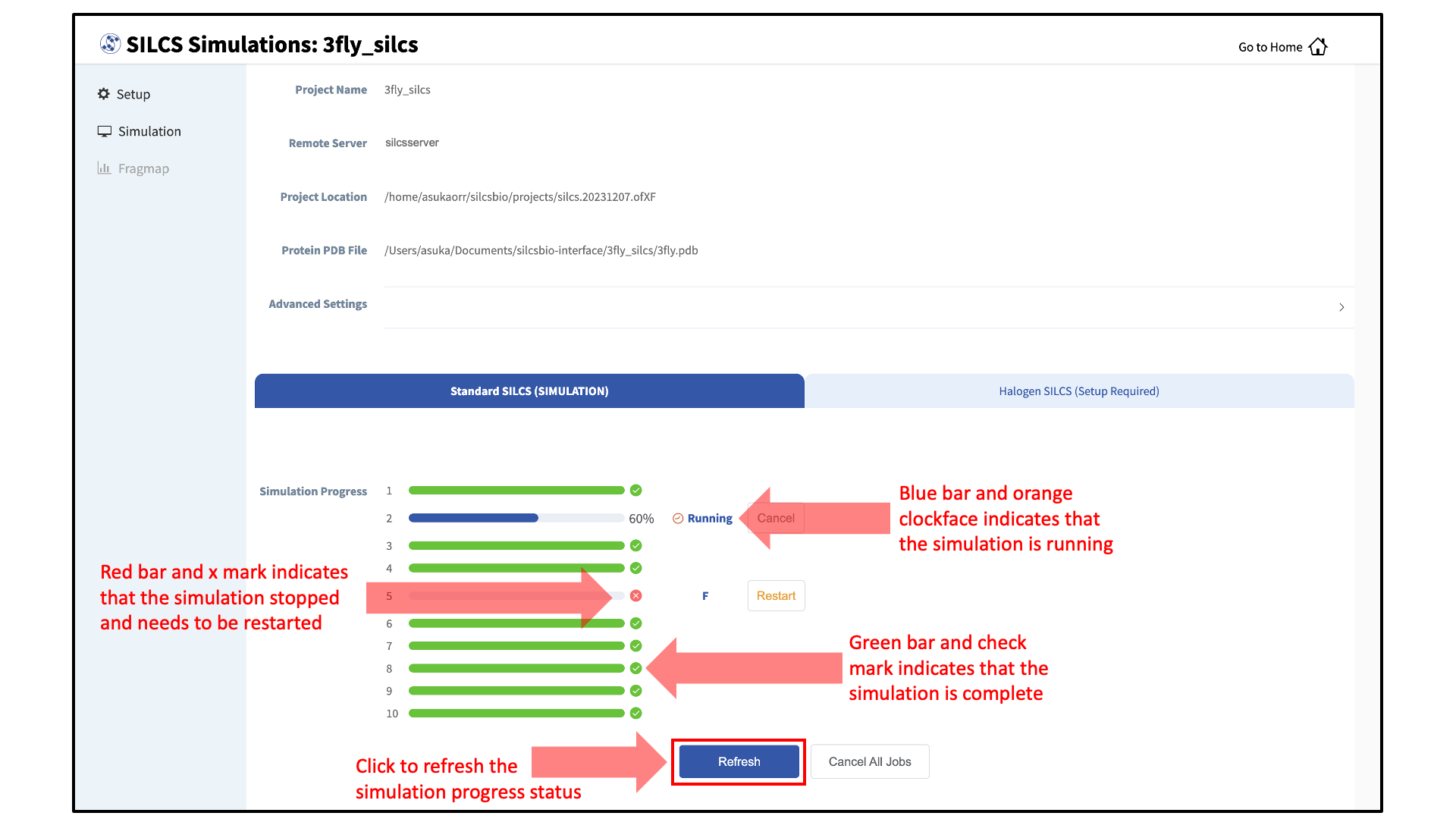
The status of each job is shown next to its progress bar: “Q” for queued, an orange clock and “Running” for running, “NA” for not submitted, and “F” for failed. When a job successfully completes, its progress bar will turn green.
Once your jobs are in progress, in either the queued or running state, you may safely quit the SilcsBio GUI or go back to the Home page to do other tasks.
If a job encounters an error or you cancel it before it finishes, its progress bar will turn red. “Restart” will appear next to the progress bar. Pressing “Restart” will resubmit the job to the queue and continue from the last cycle of the calculation so that previous progress on that job is not lost.
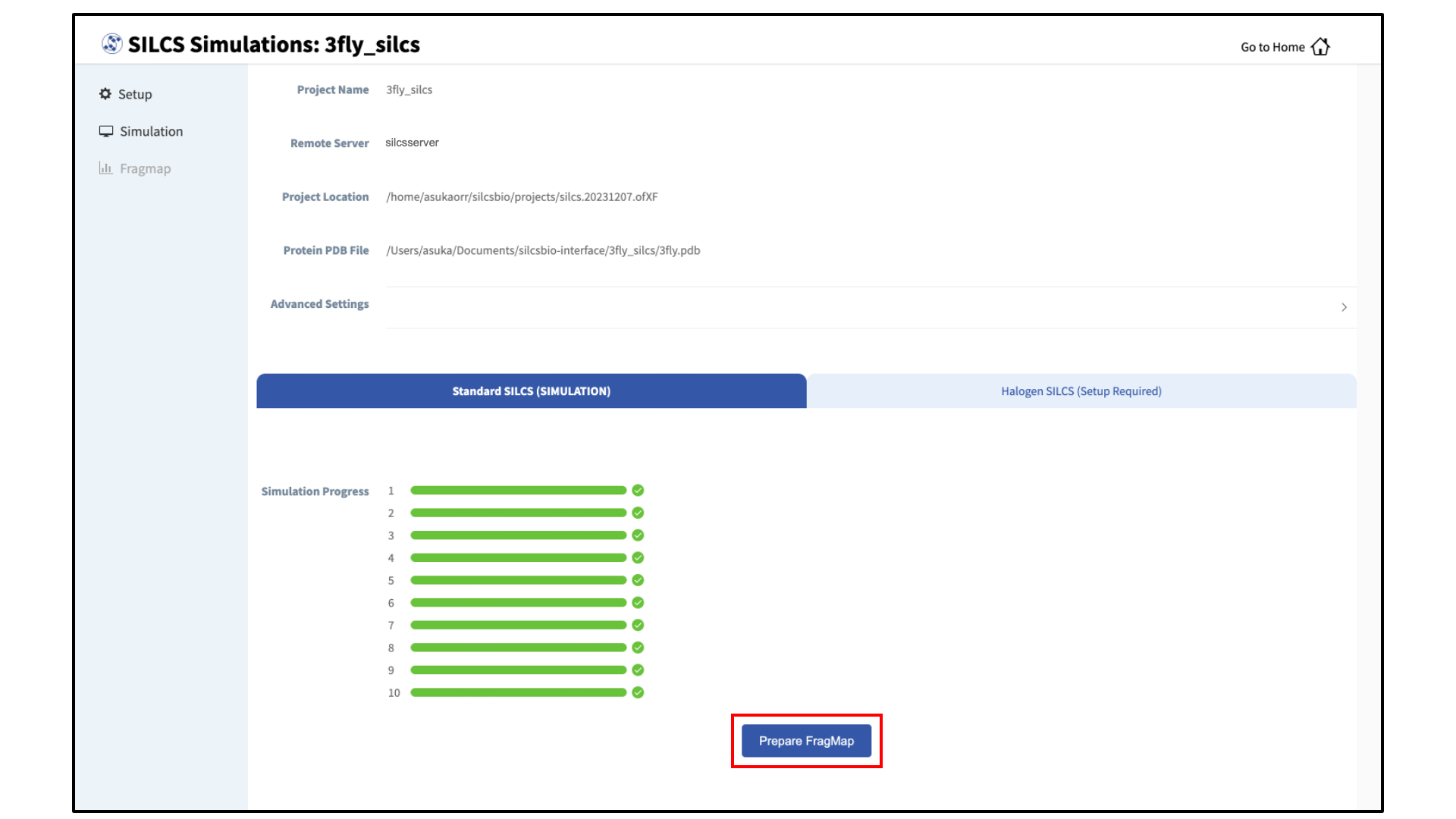
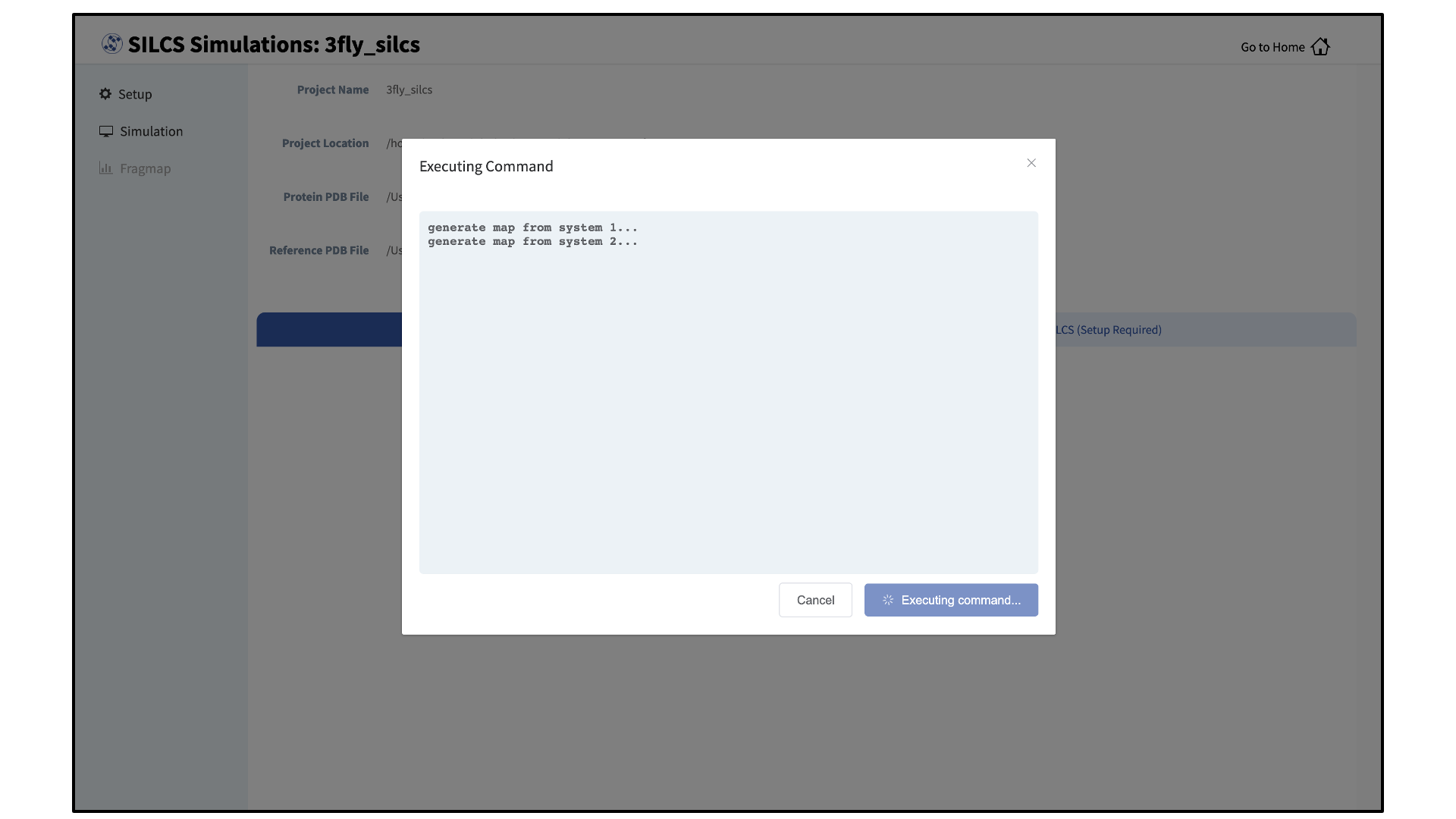
Generate FragMaps:
Once your SILCS compute jobs are finished, the GUI can be used to create FragMaps and visualize them. Green progress bars indicate successful job completion. Once all progress bars are green, the “Prepare FragMap” button will appear.
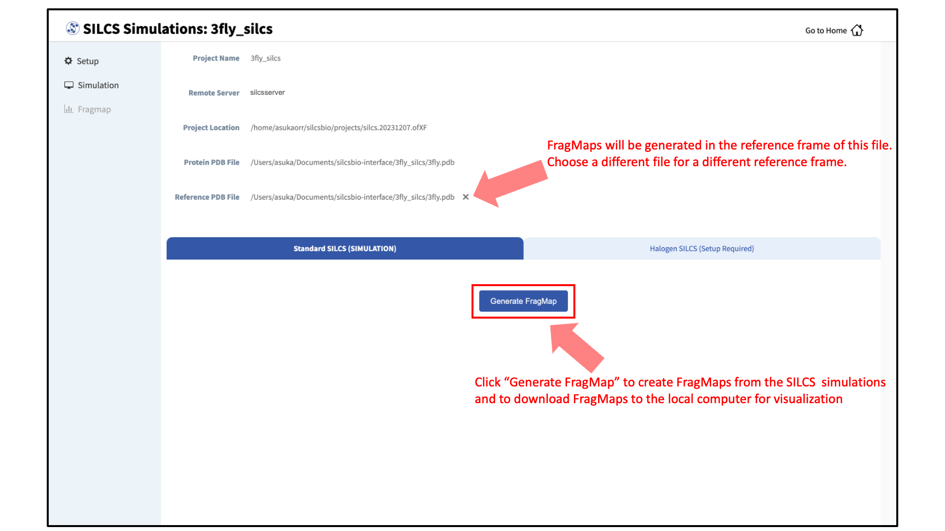
Press this button, and on the next screen, confirm your “Reference PDB File.” FragMaps will be created in the coordinate reference frame of this file. Generally, this reference PDB file is the same as the protein PDB file. A different file with the protein in a different orientation can be selected if you want to generate FragMaps relative to that orientation. Click “Generate FragMap” to generate FragMaps and download them to the local computer for visualization.
Tip
If you plan to compare FragMaps from two different protein structures, you will want to generate them with the same orientation. In that case, pre-align your input structures with each other and use these aligned coordinates as your Reference PDB Files.
Processing the GCMC-MD trajectories will take 10-20 minutes, with the GUI providing updates on progress from the server during the process.
Once completed, the GUI will automatically copy the files from the server to the local computer and load them for visualization. Please see Visualizing SILCS FragMaps for details on how to use the SilcsBio GUI, as well as external software (MOE, PyMol, VMD), to visualize SILCS FragMaps.
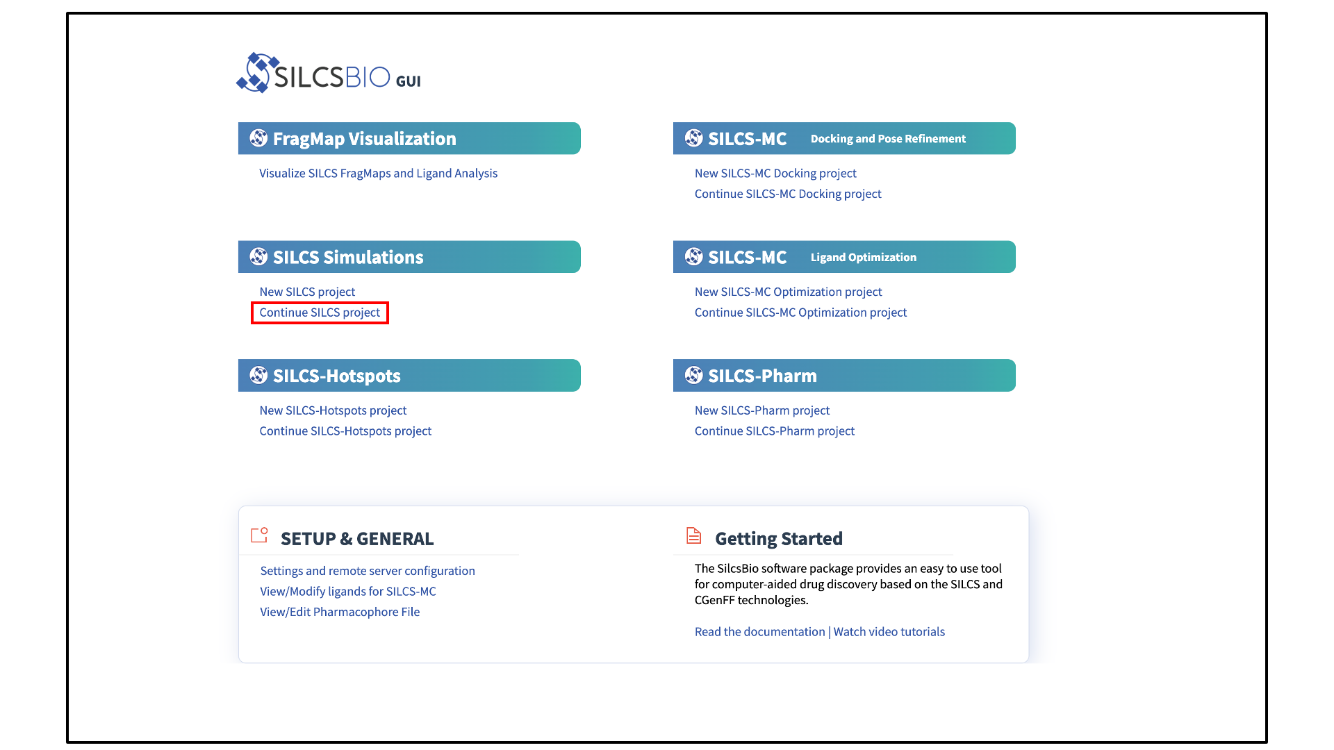
Continue SILCS projects:
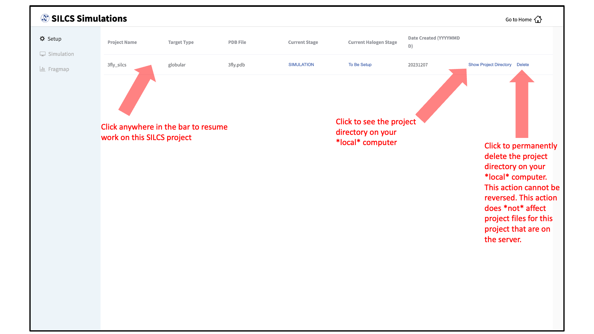
To see a full listing of all of your projects, select Continue SILCS project from the Home page. This will show the complete list of all SILCS projects you have set up on the local machine where you are currently running the SilcsBio GUI, as well as the status of each project.
To resume work on a project or check the status of associated compute jobs you previously started, simply click the project name in the list.
Data from SILCS simulations are used to pre-compute SILCS FragMaps, which are the basis for a host of functionality. The FragMaps can be used for detecting hotspots and fragment-based drug design (SILCS-Hotspots), creating pharmacophore models (SILCS-Pharm), docking ligands and refining existing docked poses (SILCS-MC: Docking and Pose Refinement), and optimizing a parent ligand (SILCS-MC: Ligand Optimization).
For additional details on SILCS, please see SILCS Simulations.
Modify Ligand for SILCS-MC
Given an input parent ligand structure, the SilcsBio GUI provides an intuitive way to modify ligands and save the modified ligand structures in Mol2 format. The resulting structures can be used as input for SILCS-MC. Ligand modifications can be built independently of any other task by choosing Modify ligand for SILCS-MC from the Home page. For instructions on how to modify ligands, please refer to Ligand Modifications Using the SilcsBio GUI.
View and Edit Pharmacophore Files
Given an existing pharmacophore file, the SilcsBio GUI provides a convenient platform to view and edit pharmacophore models. The pharmacophore file viewing and editing platform can be accessed by choosing View/Edit Pharmacophore File from the Home page. Using this tool, users can view pharmacophore models in the context of the target protein and the corresponding FragMaps, measure distances between pharmacophore features, select or deselect pharamacophore features in the pharmacophore model, adjust the feature radii, and save the modified pharmacophore model into a new pharmacophore file. For instructions on how to view and edit existing pharmacophore files, please refer to View and Edit Pharmacophore Files.
SILCS-Biologics Suite Quickstart
SILCS-Biologics builds on the SILCS technology to facilitate the screening and selection of excipients for biologics formulations. SILCS-Biologics combines the distribution of the probability of residues participating in protein–protein interactions (PPI) on the entire protein surface, determined through SILCS-PPI, with the distribution of excipients, buffers, and monoions on the surface of the protein, determined through SILCS-Hotspots. This combination allows for excipients that may block PPI, which may contribte to protein aggregation or increased viscosity, to be identified and analyzed. Such information can be used to facilitate the selection of excipients, especially in formulations that require high protein concentrations. For more information on SILCS-Biologics, please refer to SILCS-Biologics Background.
SilcsBio GUI users can access the SILCS-Biologics Suite by selecting from the menu bar.

After accessing the SILCS-Biologics Suite, the user will directly enter the New Project window. Other windows can be selected by hovering over the left sidebar and clicking on the desired option.
From the sidebar menu, SilcsBio GUI users can
Begin a new SILCS-Biologics project (New Project)
Continue or monitor existing SILCS-Biologics projects (Project List)
If continuing a SILCS-Biologics project (Project List), SilcsBio GUI users can also
Finalize the setup for an existing SILCS-Biologics project (Setup)
Monitor the progress of an existing SILCS-Biologics project (Progress)
Visualize the results of an existing SILCS-Biologics project (Visualization)
Details on how to use SILCS-Biologics through the SilcsBio GUI are provided below.
SILCS-Biologics Using the GUI
To begin a new SILCS-Biologics project, follow these steps:
Begin a new SILCS-Biologics project:
By default, the user will directly enter the New Project page in which new SILCS-Biologics projects can be initiated. If the user is in a different page, the New Project page can be accessed by hovering over the left sidebar and selecting New Project.
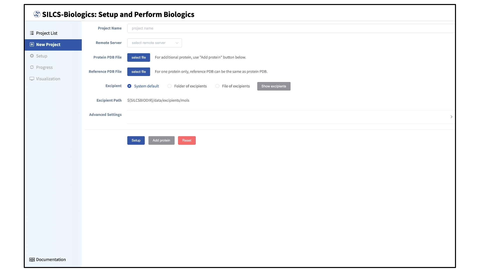
Enter a project name, select the remote server, and upload input files:
Enter a project name and select the remote server where compute jobs will run. Next, select a PDB file containing the coordinates of the target protein as described in File and Directory Selection.
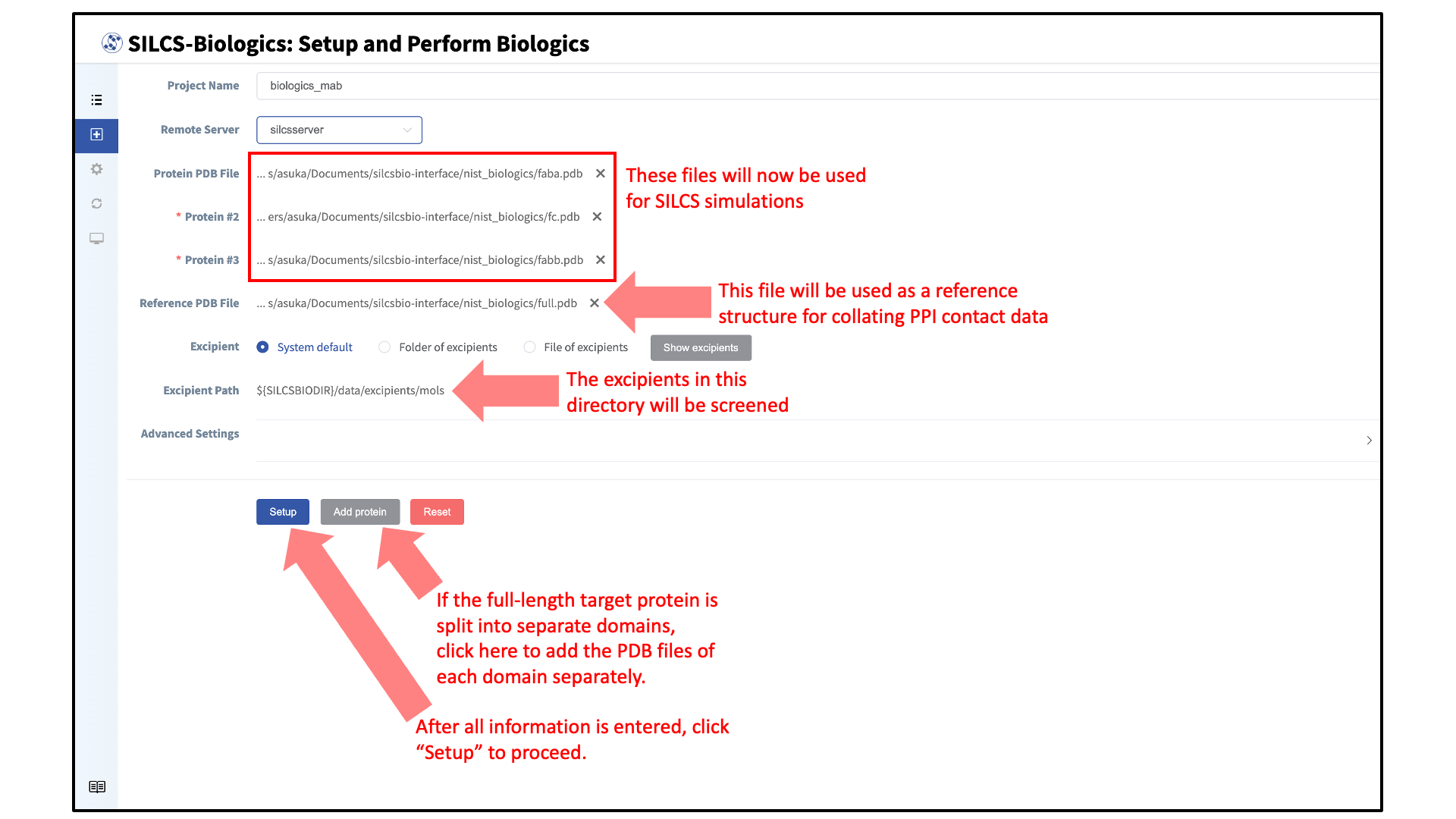
If the target protein is large and contains distinct domains (e.g., monoclonal antibodies), the full-length protein may be split into its separate domains for computational expediency. In this case, each domain should be entered as a separate PDB file. To add additional PDB files, click the “Add protein” button at the bottom of the page for each additional PDB file.
Additionally, enter a reference structure of the full-length target protein. This structure will be used a reference structure for collating PPI contact data as well as for excluding surface-exposed amino acids in individual input protein domains that are in fact buried in the context of the full-length protein. If only one PDB file was entered for “Protein PDB File”, then the same PDB file should be used for “Reference PDB File”.
Note
If you do not have the full-length structure of the target protein, but only have the structures of individual domains, then the full-length protein structure should be constructed using other molecular modeling tools (such as homology modeling software). The modeled full-length structure can then be used as the “Reference PDB File”.
Alternatively, the positions of the individual domains in the context of the full-length protein can be estimated through a simple structural alignment to a known full-length homologous crystal structure, and the resulting superimposed structure of the individual domains can be saved and used as the “Reference PDB File”.
Warning
Dividing the target protein into domains entails independent SILCS simulations for each of the domains. E.g., for SILCS-Biologics runs with
prot1,prot2, andprot3specified (3 domains) 3 \(\times\) 10 SILCS simulations will be performed rather than 1 \(\times\) 10 SILCS simulations. If sufficient compute nodes are available to run all SILCS simulations for all domains simultaneously, the SILCS simulations for the target protein will be completed sooner using the domain approach than running SILCS simulations of the full-length protein. However, using the domain approach may consume more CPU/GPU hours.The SilcsBio GUI provides a default set of excipients for screening (“System default”). If a custom set of excipients is desired, click the “Folder of excipients” (if excipients are stored as individual Mol2 or SD files in a folder) or “File of excipients” (if all excipients are stored in one SD file) radio button next to Excipient.
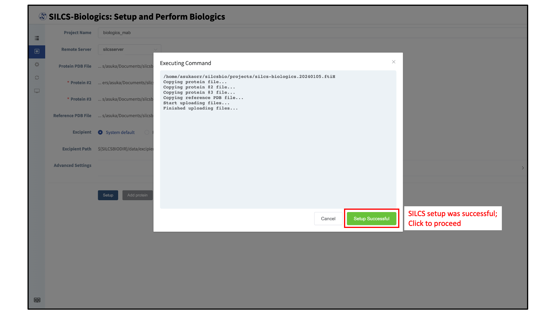
Set up SILCS-Biologics simulations:
Once all information is entered, click the “Setup” button at the bottom of the page. The GUI will contact the remote server and upload the input files specified in the previous step. A green “Setup Successful” button will appear once the process has successfully completed. Press this button to go to the next step.
Launch SILCS-Biologics simulations:
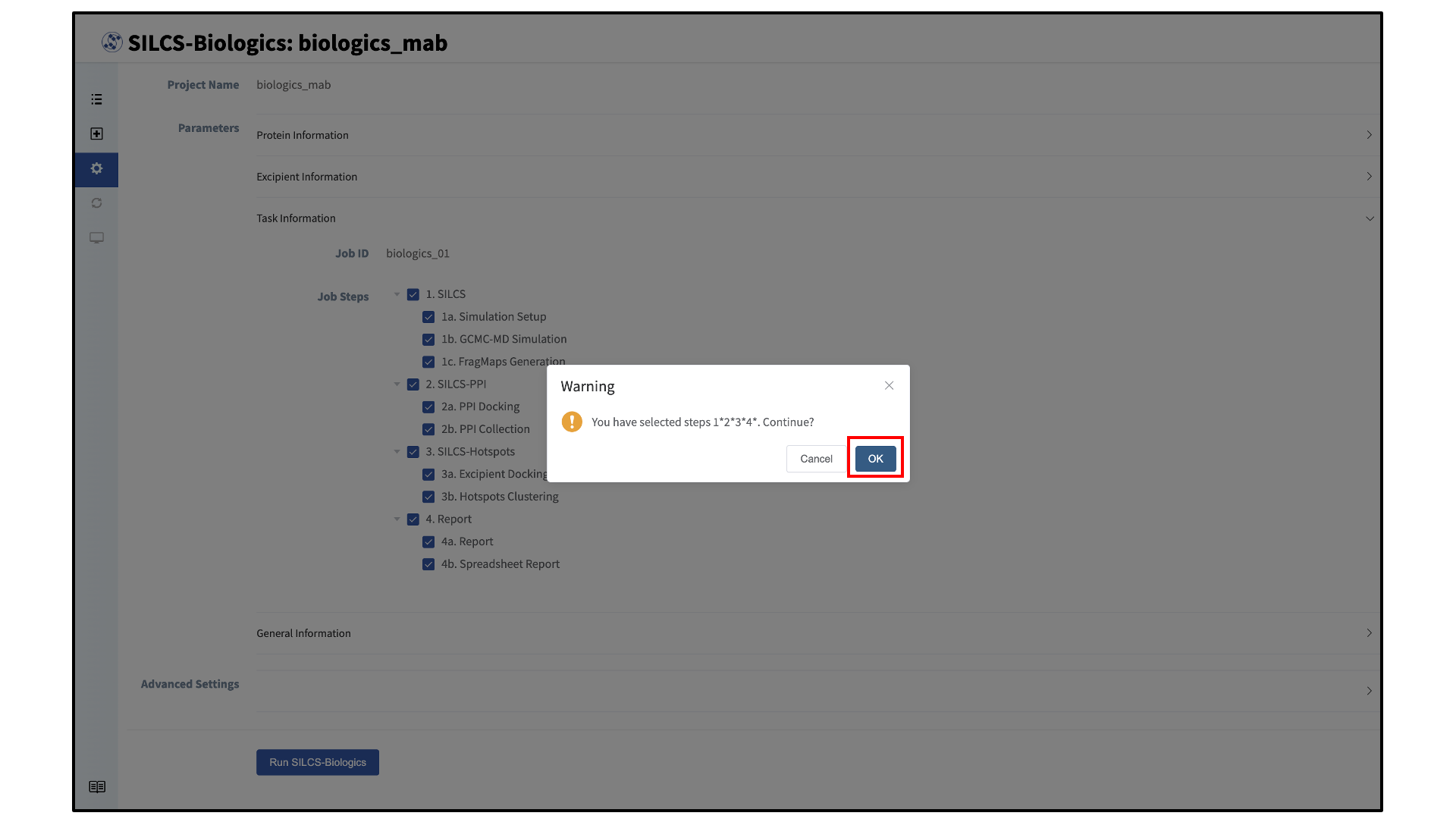
Your SILCS-Biologics simulations can now be started by clicking the “Run SILCS-Biologics” button at the bottom of the page. SILCS-Biologics may be run in a stepwise fashion if desired. To view and toggle on/off SILCS-Biologics tasks, click “Task Information”.
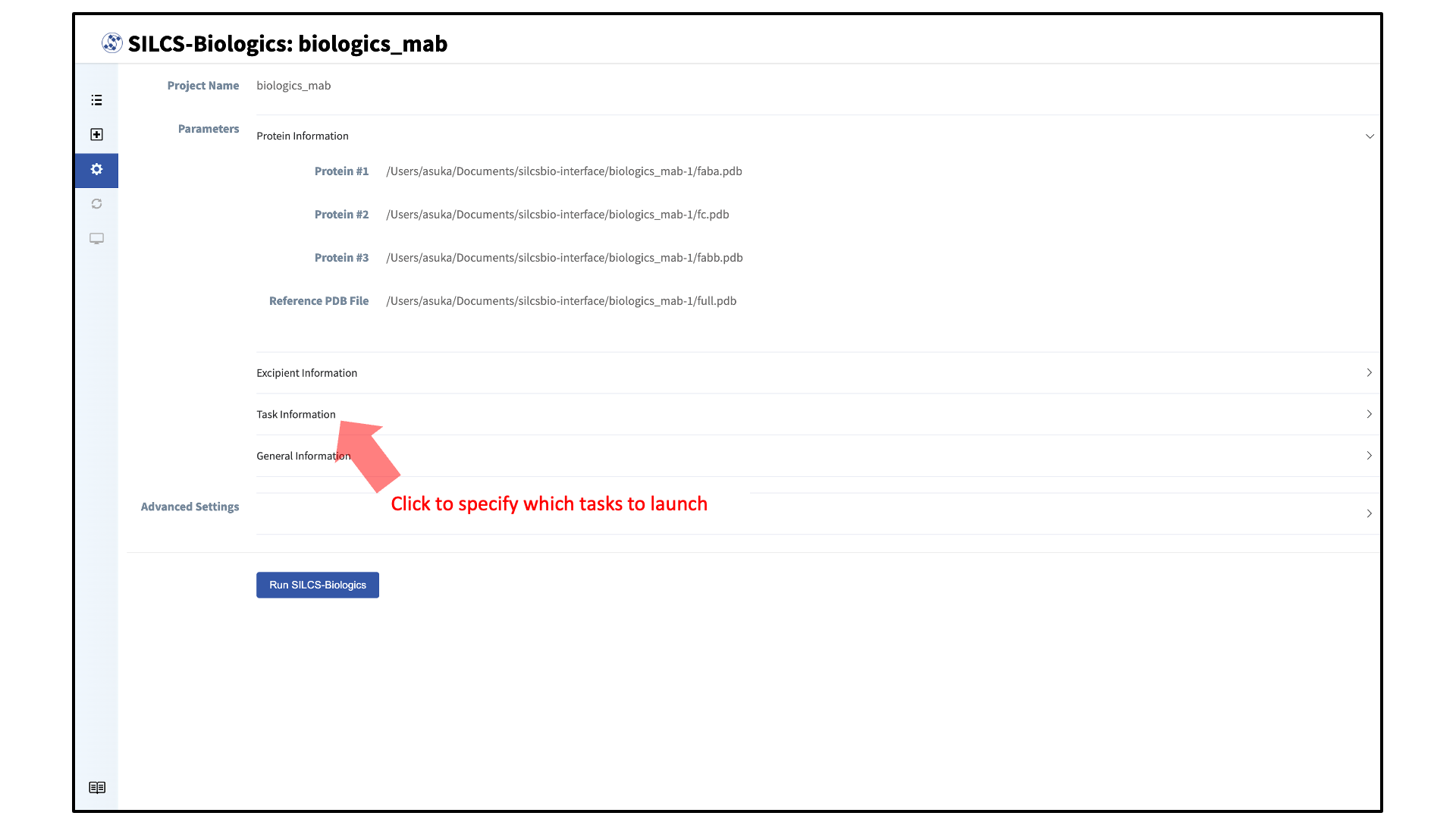
Finer control at the level of the smaller subtasks can also be requested. Note that the tasks and subtasks must be run sequentially (e.g., Step 1a must be run before Step 1b, and Step 1* must be run before Step 2*). By default, all tasks will be run.
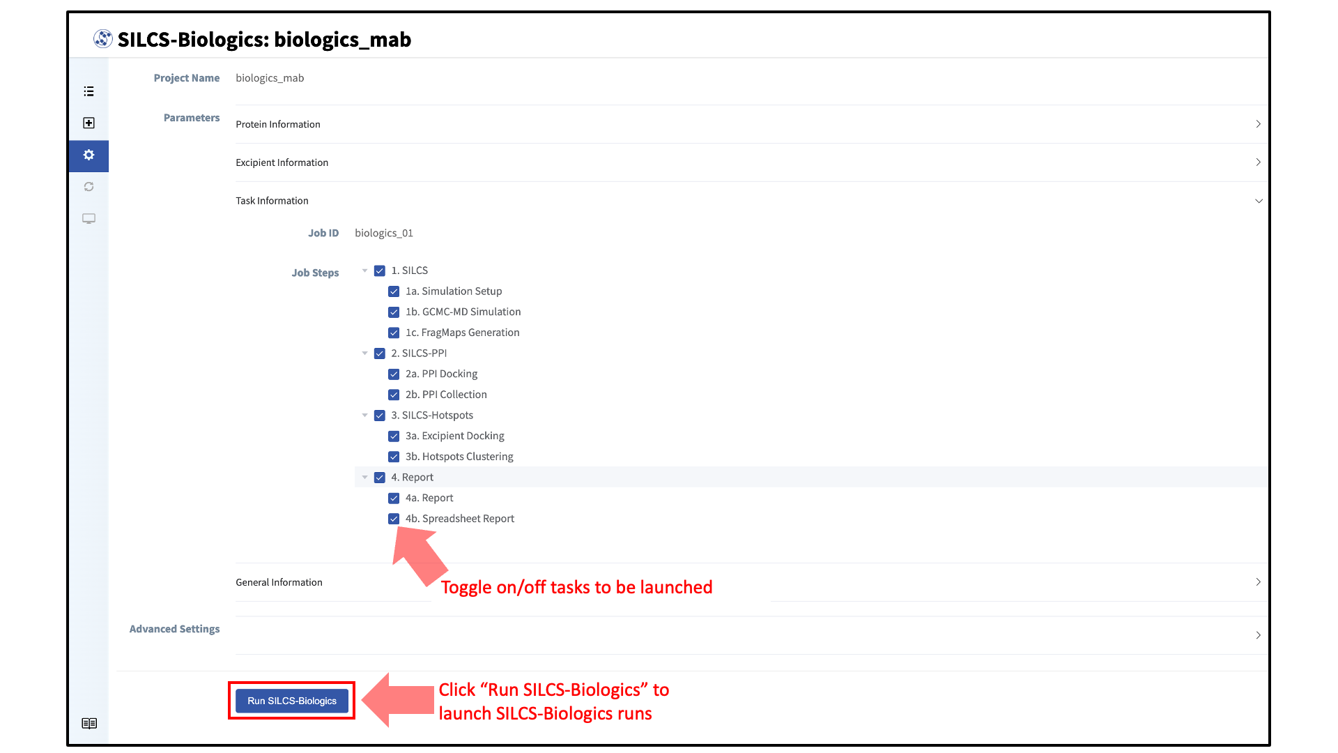
After clicking the “Run SILCS-Biologics” button, the SilcsBio GUI will prompt the user to confirm the tasks to be submitted with a warning window. Click “OK” to confirm the selected tasks. To return to the task selection page, click “Cancel”.
After confirming the tasks to be performed with clicking “OK” on the warning window, compute jobs will be submitted to the queueing system on the server.
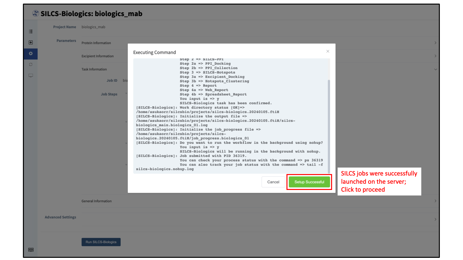
A green “Setup Successful” button will appear once the jobs are successfully launched on the server. Click this button to proceed.
Monitor SILCS-Biologics tasks:
The progress of each SILCS-Biologics task can be monitored by clicking “Progress” in the sidebar menu. Alternatively, the “Progress” page can be accessed by going to the “Project List” page through the sidebar menu and clicking on the desired SILCS-Biologics project if the project’s SILCS-Biologics simulations have already been submitted. The SilcsBio GUI will also automatically take you to the “Progress” page after clicking “Setup Successful” in the previous step.
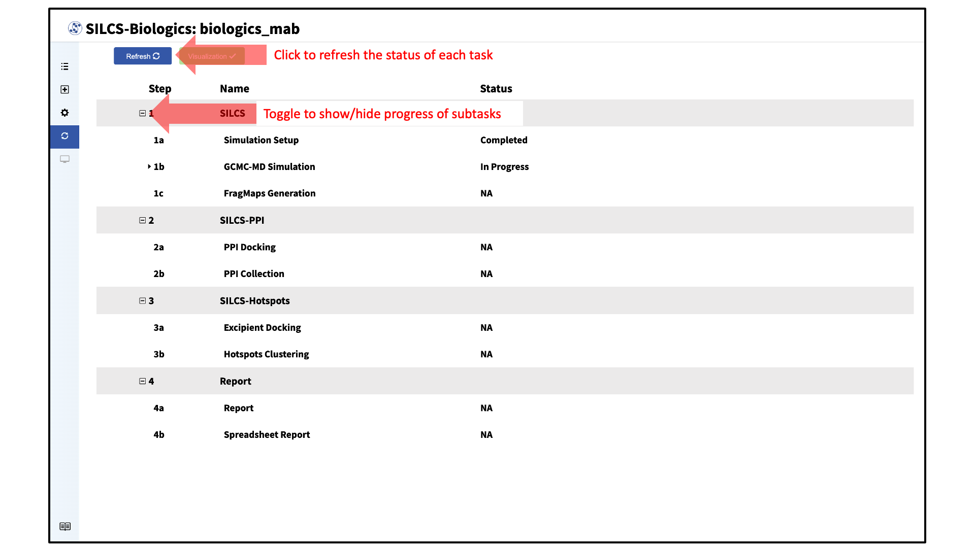
In the “Progress” page, the status of each task can be refreshed by clicking the “Refresh” button at the top left of the page. The progress of each subtask can also be viewed by toggling “+/–”.
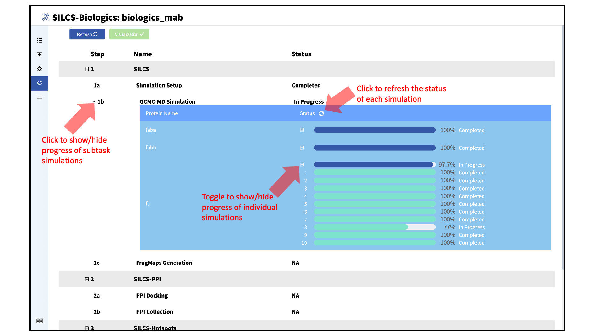
For each subtask step involving simulations (SILCS simulations, SILCS-PPI docking, and SILCS-Hotspots excipient docking), the progress of individual simulations can also be viewed by clicking the dropdown menus and toggling “+/–”.
Download and visualize SILCS-Biologics results:
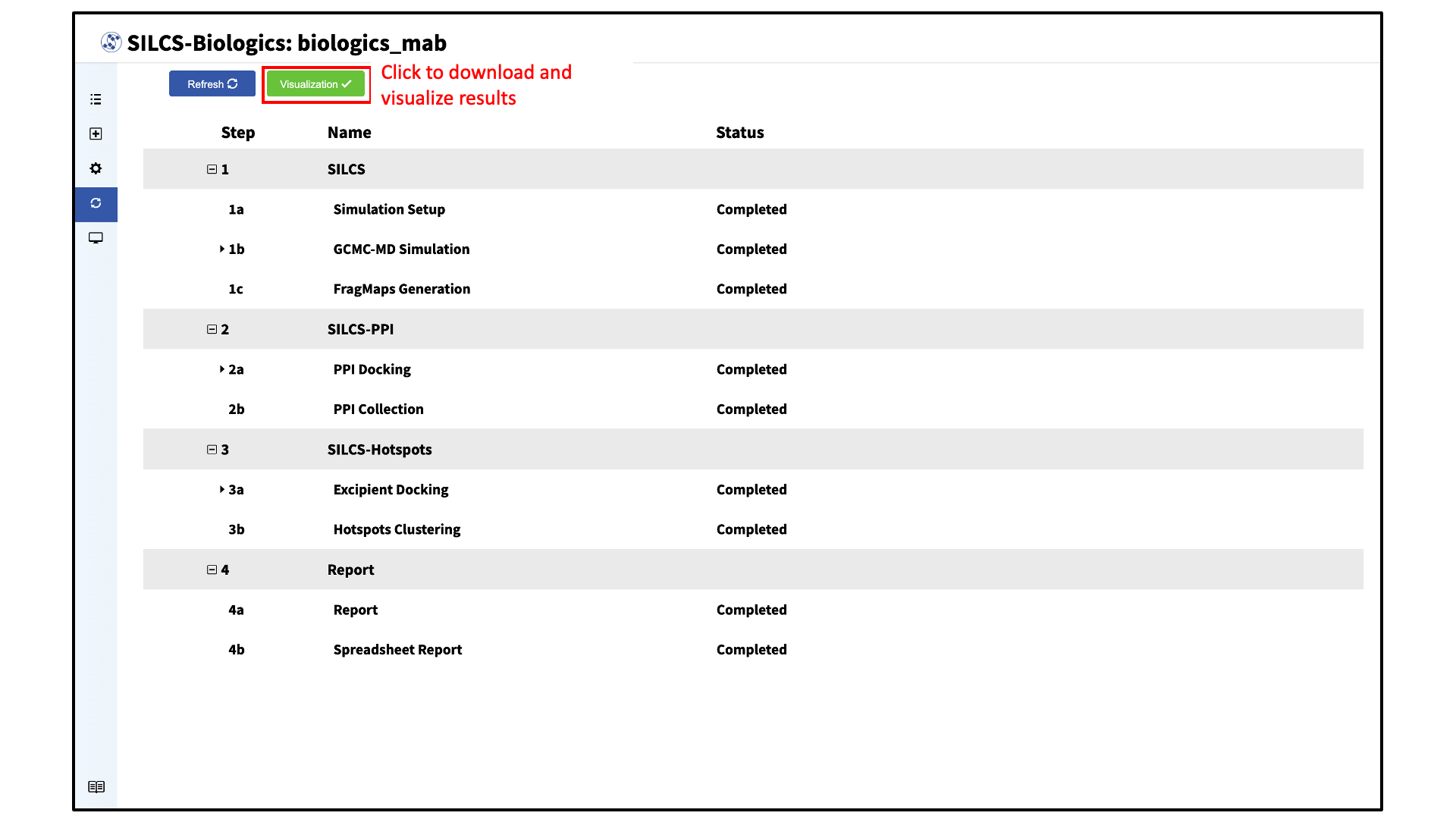
Once all SILCS-Biologics tasks are complete, the “Status” column on the Progress page for all tasks will be marked “Completed” and the green “Visualization” button at the top of the page will become active.
Click the green “Visualization” button to download the results from the remote server.
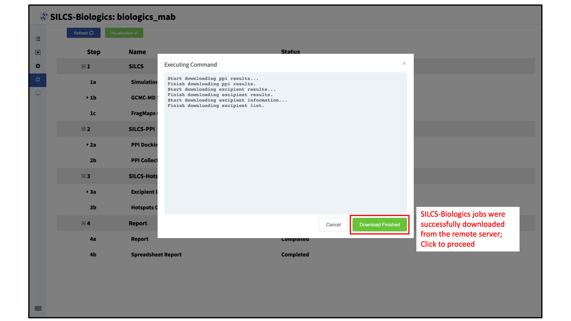
A window will appear with the download progress. After the results are successfully downloaded, the GUI will automatically update with a green “Download Finished” button. Click the “Download Finished” button to visualize the results.
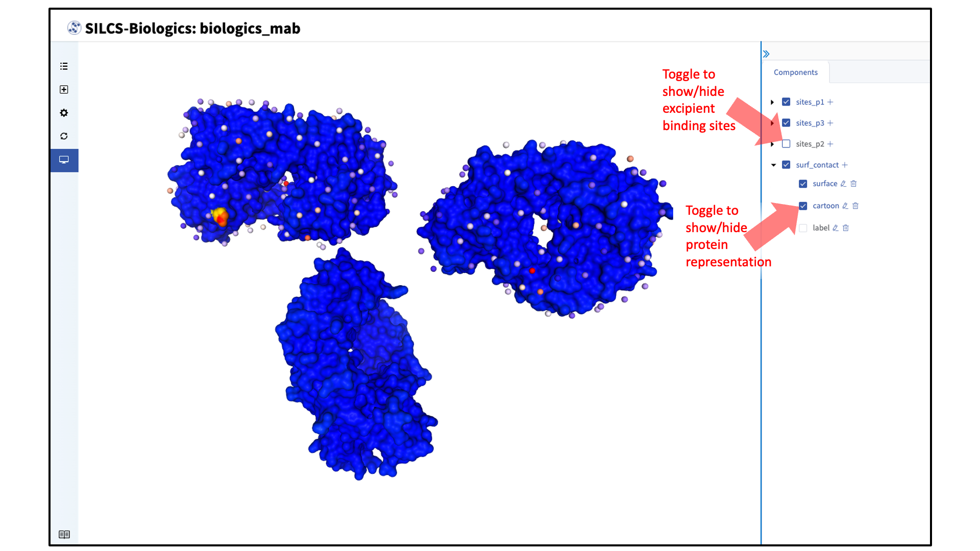
The SILCS-Biologics results (protein–protein interaction preference [PPIP] and excipient binding sites) can now be visualized for the target protein. The target protein is shown in surface representation, by default, with regions of high PPIP (regions prone to self-aggregation) colored red (PPIP score of 1) and regions with low PPIP colored blue (PPIP score of 0). In the example case shown in the figures, SILCS-Biologics was applied to NISTmAb, which is not prone to aggregation. This is reflected by the primarily blue surface shown. Excipient binding sites are shown in vdW representation, with more energetically favorable binding sites colored red and less energetically favorable (site LGFE of greather than -2 kcal/mol) colored blue. Representations of the protein can be customized under “surf_contact”. Representations of the excipient binding sites can be customized under “sites_p<protein number>”, with <protein number> indicating the protein PDB file entered. In the example case shown in the figures, sites_p1 corresponds to faba.pdb (“Protein PDB File”), sites_p2 corresponds to fc.pdb (“Protein #2”), and sites_p3 corresponds to fabb.pdb (“Protein #3”).
Generate formulation report:
The SILCS-Biologics data can help connect experimental observables to the molecular details of protein–excipient interaction. In doing so, these data can help both rationalize known trends for existing data on excipients and guide the selection of new excipients for additional testing. With regard to the former, the most straightforward approach is to compare available experimental data to SILCS-Biologics metrics and note correlations. The SilcsBio GUI provides a platform to generate formulation reports and chart correlations between experimental data and SILCS-Biologics metrics.
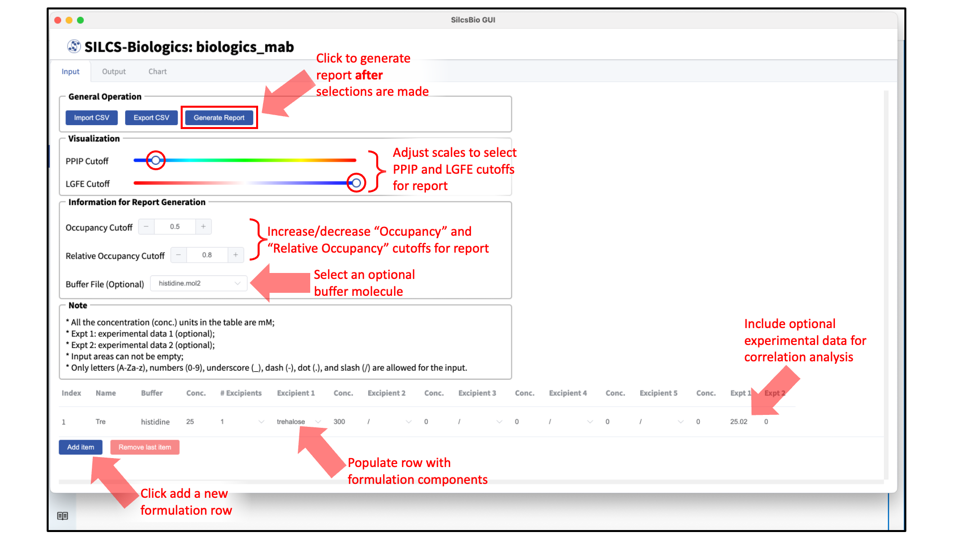
To generate a report, first enter the details on formulations of interest at the bottom of the page. These details are:
(1st column, “Name”) the name of the formulation,
(2nd column, “Buffer”) the buffer molecule if applicable,
(3rd column, “Conc.”) the concentration in mM of the buffer molecule if applicable,
(4th column, “# Excipients”) the number of excipients in the formulation excluding the buffer molecule,
(5th column, “Excipient 1”) the first excipient in the formulation,
(6th column, “Conc.”) the concentration in mM of the first excipient in the formulation,
(7th, 9th, 11th, or 13th column, “Excipient N”) the Nth excipient in the formulation if applicable,
(8th, 10th, 12th, or 14th column, “Conc.”) the concentration in mM of the Nth excipient if applicable,
(15th column, “Expt 1”) the first experimental data for the formulation if available, and
(16th column, “Expt 2”) the second experimental data for the formulation if available.
To add additional formulations to the analysis, click the “Add item” button at the bottom of the page. To remove the last formulation entered, click the red “Remove last item” button. Alternatively, this information can be uploaded all at once by importing a a CSV file using the “Import CSV” button under “General Operation” at the top of the page. The formulations can additionally be saved into a CSV file using the “Export CSV” button in the same location.
Next, specify cutoff values to include/exclude bindings sites for analysis in the formulation report.
The PPIP and LGFE cutoffs can be selected using the selection scale under “Visualization”. The colors on the scale correspond to the colors shown in the visualization window. Using the LGFE criterion, for an excipient binding site to be counted, the excipient(s) in a given formulation must have an LGFE less than the LGFE cutoff. Using the PPIP criterion, for an excipient binding site to be counted, the residues in proximity to the binding site must have a PPIP greater than the PPIP cutoff.
The occupancy and relative occupancy cutoffs can be selected under “Information for Report Generation”. Using the occupancy criterion, for an excipient binding site to be counted, the excipient(s) in a given formulation must have an occupancy greater than the occupancy cutoff. Using the relative occupancy criterion, for an excipient binding site to be counted, the excipient(s) in a given formulation must have a relative occupancy greater than the relative occupancy cutoff.
Note
The occupancy of an excipient at a given binding site is a function of its LGFE and concentration:
\[\textrm{occupancy} = [L]/([L] + K_d)\]where \(K_d\) is the dissociation constant such that \(LGFE = RT \ln {K_d}\) and \([L]\) is the concentration of the excipient in the formulation with unit mM. The occupancy has a range of 0 to 1 with 1 indicating that the excipient has a high probability of binding at the site and 0 indicating that the excipient has minimal probability of binding at the site.
Finally, select the Mol2 file of the buffer molecule if applicable in the dropdown menu under “Information for Report Generation”.
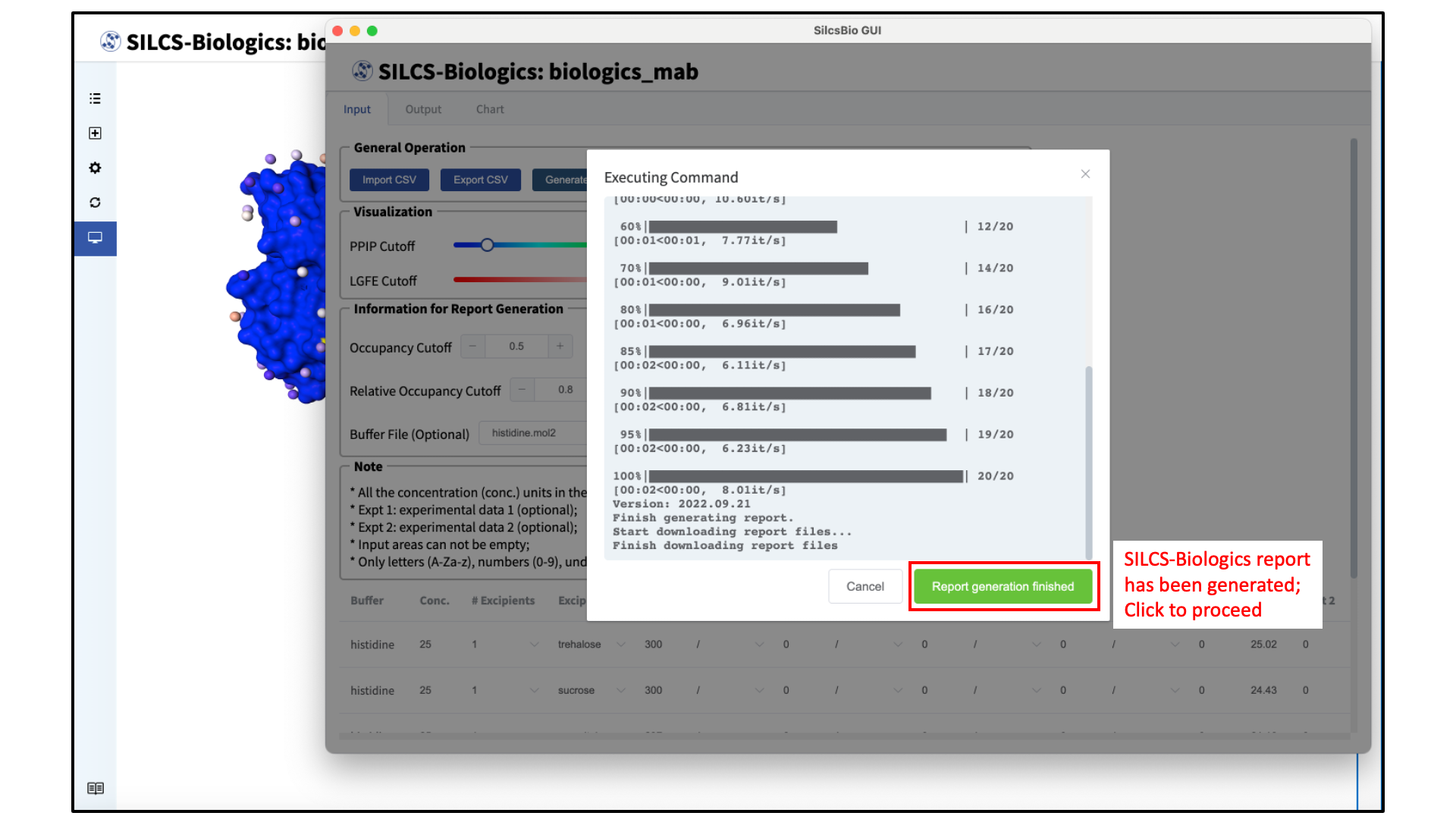
Once all selections have been made, click the “Generate Report” button at the top of the page, under “General Operation”. The SilcsBio GUI will initiate calculations to generate SILCS-Biologics metrics based on the specified formulations and cutoffs. Upon completion of the calculations and report generation, a green “Report generation finished” button will appear. Click on the green “Report generation finished” button to view the output.
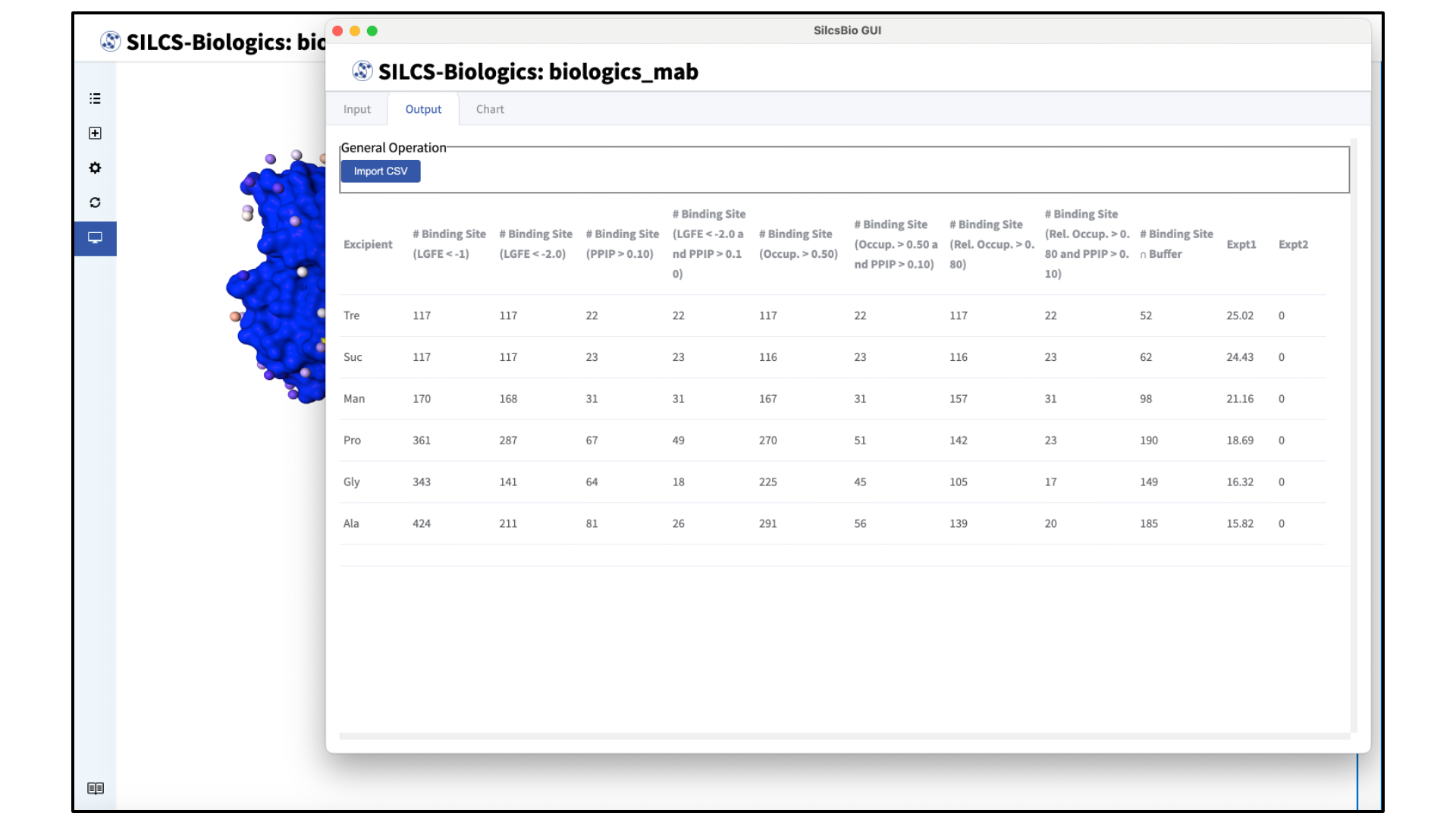
View formulation report output:
After the calculations are completed and the report is generated, the GUI will automatically display a table of SILCS-Biologics metrics for each formulation entered in the previous step. Data from an existing CSV output can also be uploaded using the “Import CSV” button in the “Output” tab.
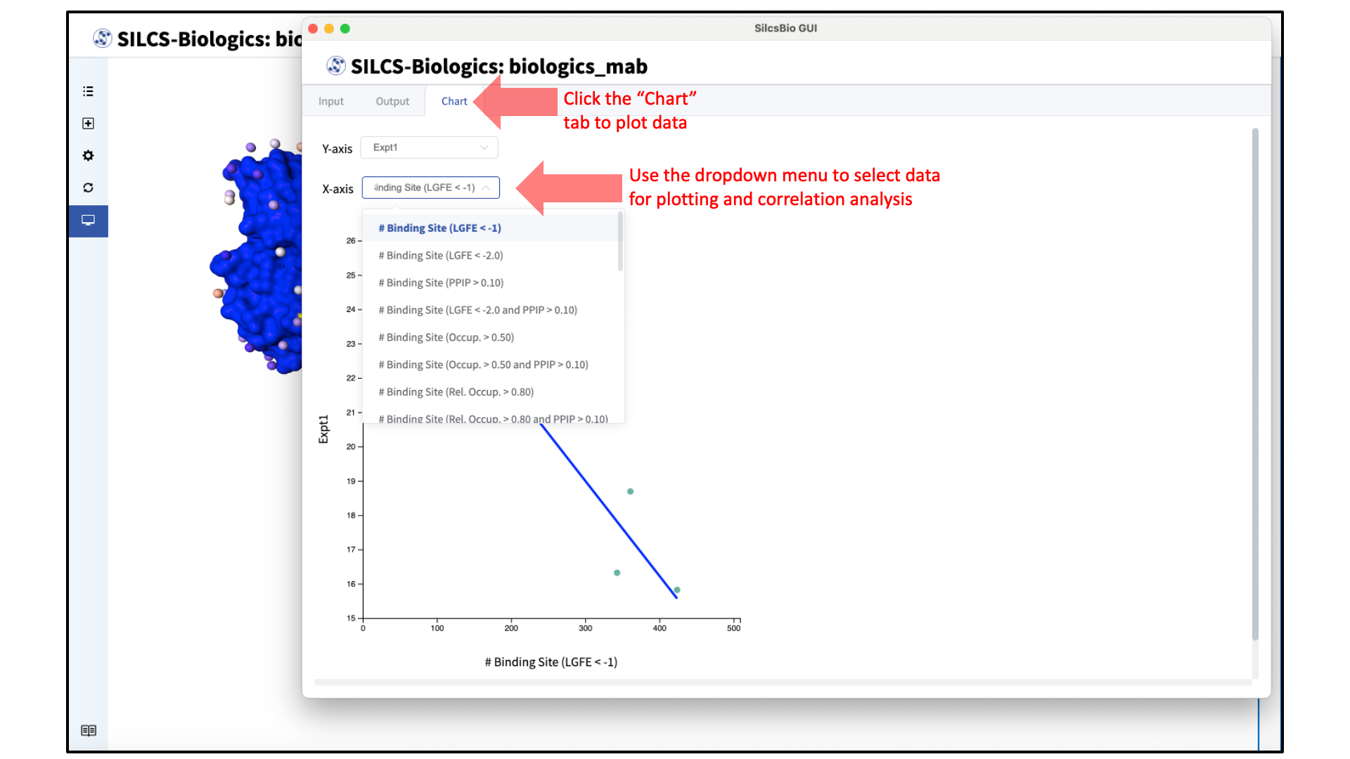
To plot the SILCS-Biologics metrics against experimental data, click the “Chart” tab and select the Y-axis (choose between experimental data entered for “Expt1” and “Expt2” in the previous step) and X-axis (choose SILCS-Biologics metrics generated based on specifications selected in the previous step).
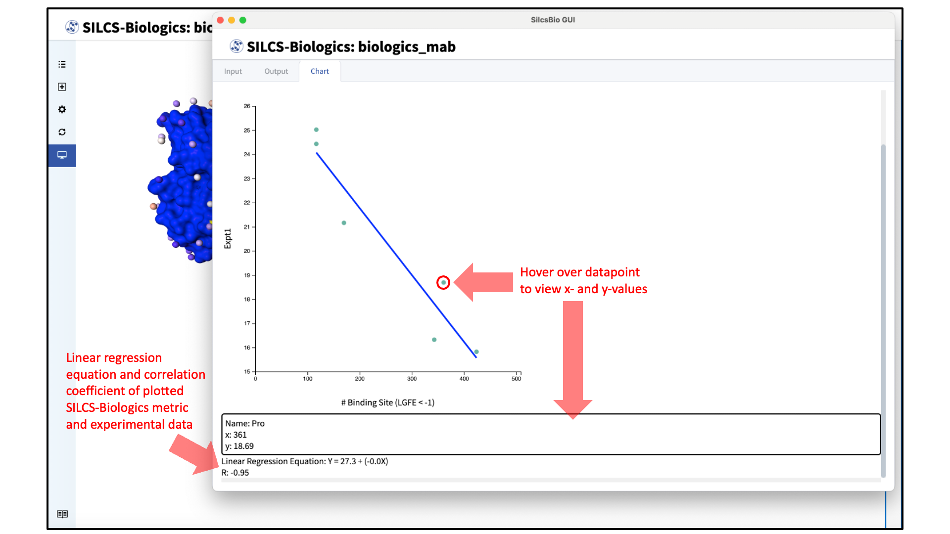
The plot will appear automatically with the linear regression equation and correlation between the experimental data and the SILCS-Biologics metric (“R”) below the plot. Specific values and the formulation name of each datapoint can be viewed by hovering over the datapoint.
SSFEP Suite Quickstart
Single Step Free Energy Pertubation (SSFEP) is a rapid method for evaluating relative binding affinities, enabling the assessment of numerous modifications to a parent ligand. Additional information on SSFEP can be found in SSFEP: Single Step Free Energy Perturbation.
SilcsBio GUI users can access the SSFEP Suite by selecting from the menu bar.

The SSFEP Suite Home page provides easy access for users to
Begin a new SSFEP project (New SSFEP project)
Continue an existing SSFEP project (Continue SSFEP project)
The SSFEP Suite also provides convenient access to general tools under SETUP & GENERAL at the bottom of the page.
For additional information on these tools, please click on their links. Details on how to use the SSFEP Suite in the SilcsBio GUI are provided below.
SSFEP Simulations Using the GUI
To begin a new SSFEP project, follow these steps:
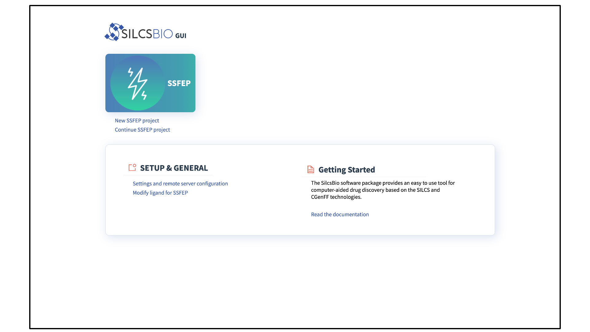
Begin a new SSFEP project:
Select New SSFEP project from the Home page.
Enter a project name, select the remote server, and upload input files:
Enter a project name, and select the remote server where compute jobs will run.
Note
Typical SSFEP simulations produce output files in excess of 20 GB, so please select a project location file folder with appropriate storage capacity. The project location can be changed by entering the “Settings and remote server configuration” page from the “Home” page and changing the “Project Directory” field as described in Remote Server Setup.
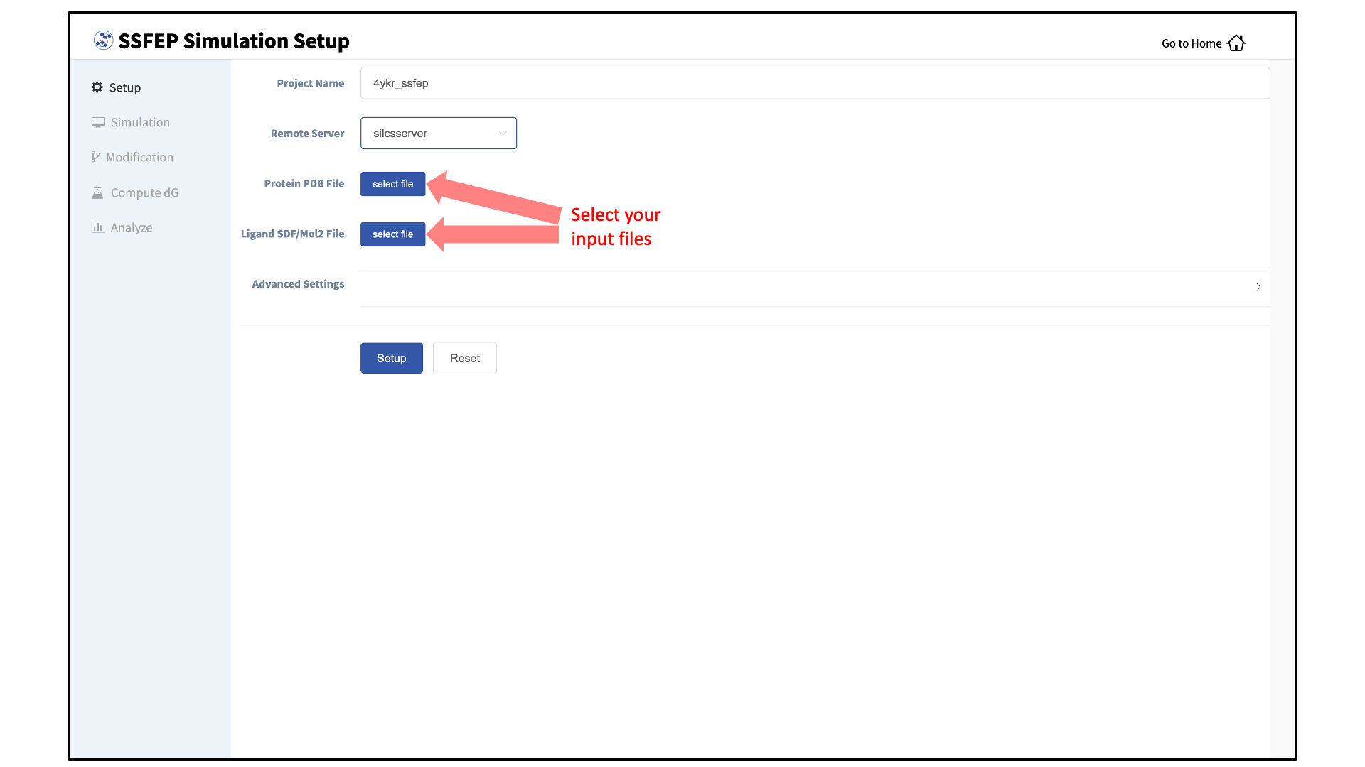
Next, select a protein PDB file and a ligand file as described in File and Directory Selection. The ligand should be aligned to the binding pocket in the accompanying protein PDB file. We recommend cleaning your PDB file before use, incuding keeping only those protein chains that are necessary for the simulation, removing all unnecessary ligands, renaming non-standard residues, filling in missing atomic positions, and, if desired, modeling in missing loops.
If the GUI detects missing non-hydrogen atoms, non-standard residue names, or non-contiguous residue numbering, it will inform the user and provide a button labeled “Fix?”. If this button is clicked, a new PDB file with these problems fixed and with
_fixedadded to the base name will be created and used in the SSFEP simulation.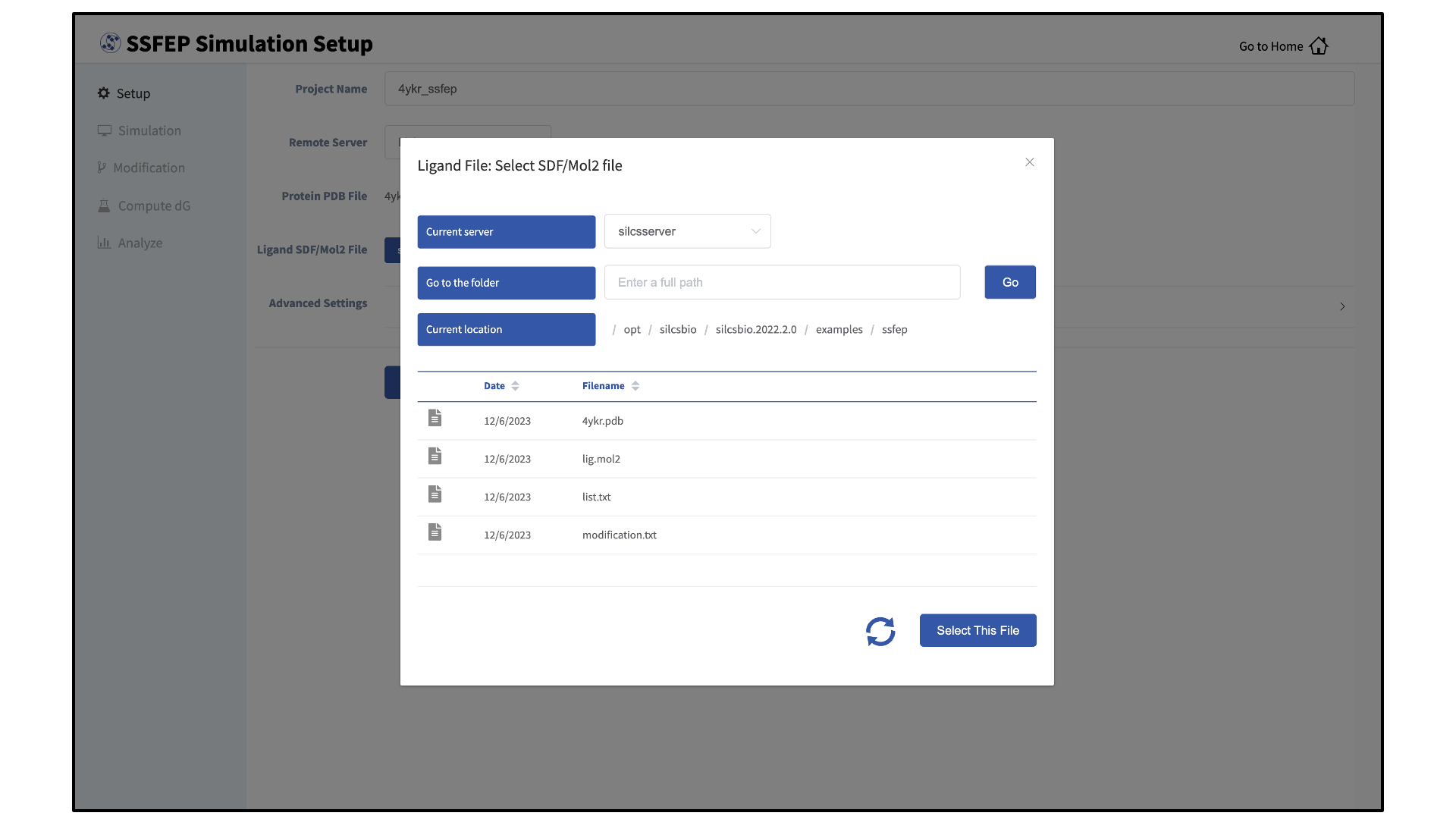
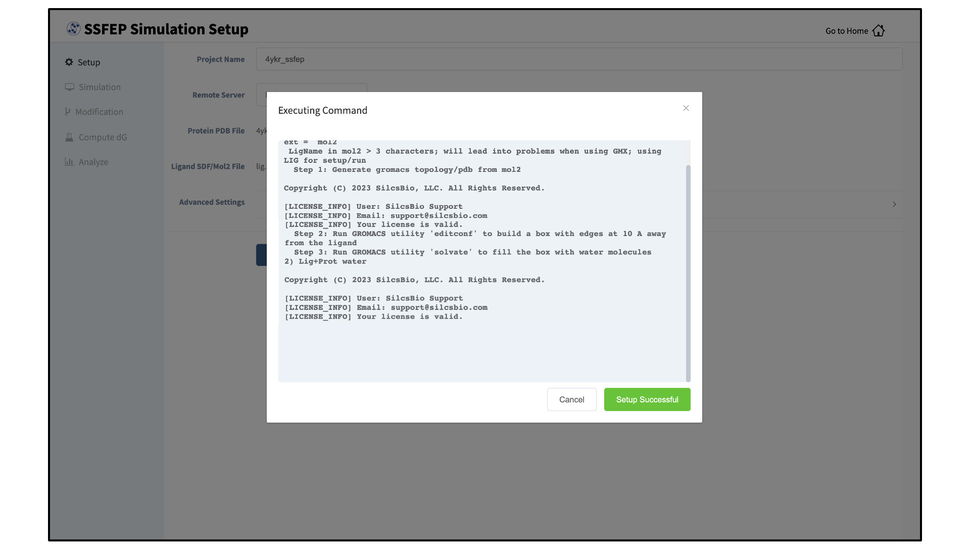
Set up SSFEP simulations:
Once all information is entered correctly, press the “Setup” button at the bottom of the page. The GUI will contact the remote server and perform the SSFEP setup process.
During setup, the program automatically performs several steps including building the topology of the simulation system and creating metal-protein bonds if metal ions are found. To complete the entire process may take up to 10 minutes depending on the system size. A green “Setup Successful” button will appear once the process has successfully completed. Press this button to proceed.
Select ligand modifications:
You can now prepare your ligand modifications with the “Add Ligand Modifications” button.
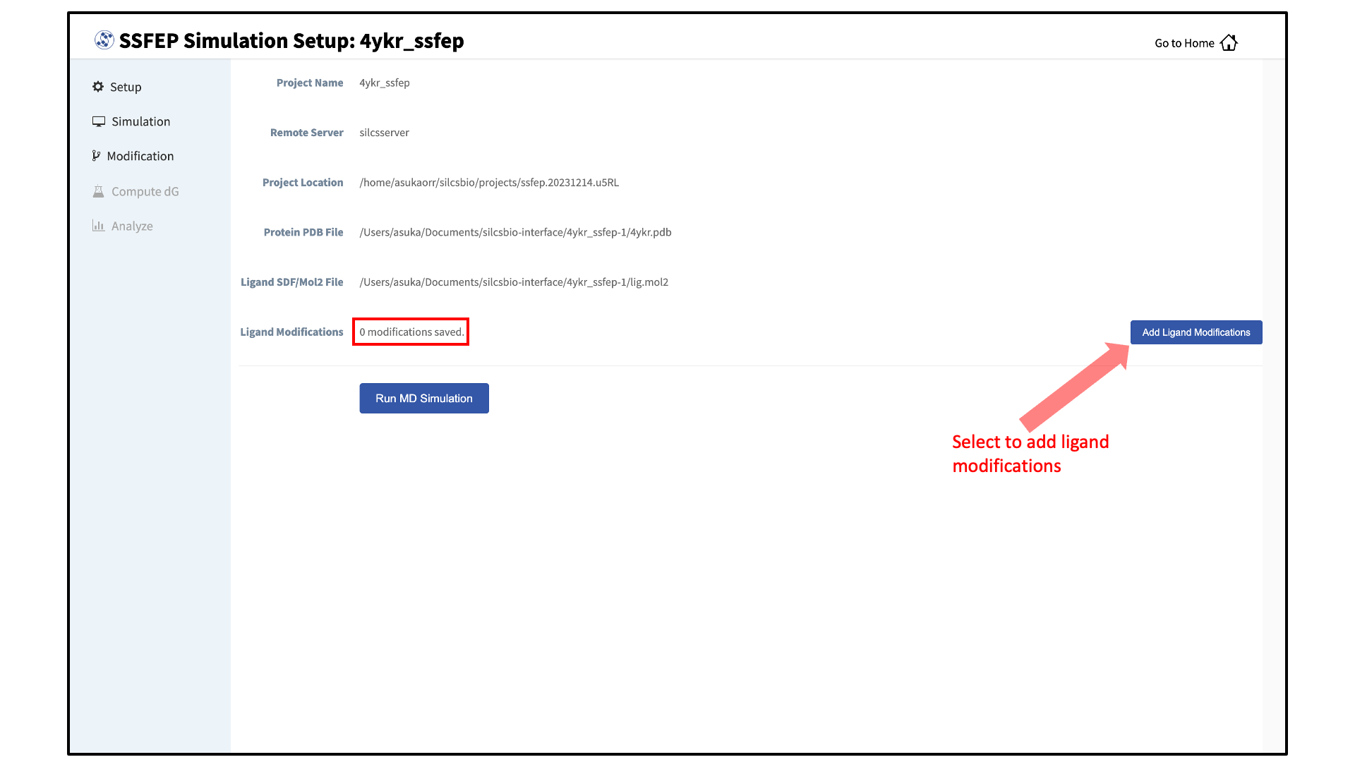
There are two major modification types, Substitution and Replacement, available in the GUI. Substitution is used to substitute a hydrogen with another functional group. Replacement is used to replace an atom in a ring with another functional group that preserves the ring.
In the visualization window, select the atom to be modified. Then, select your desired modifications from the “Substitution” or the “Replacement” tab in the right-hand panel. Pressing the “Save” button in the panel will update your list of modifications.
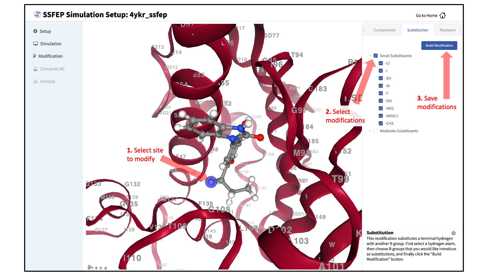
The list of modification types in the GUI covers a broad range of chemical functionality. Custom modifications can be made using the Command Line Interface (CLI) as detailed in SSFEP: Single Step Free Energy Perturbation.
Review selected ligand modifications:
Use the “Review” tab to confirm your desired modifications. Valid modifications will have a small Image icon as well as a small Trash Can icon. Clicking on the Image icon will show the modification in the center panel. Clicking on it again will show the parent ligand. Clicking on the Trash Can icon will delete the proposed modification from your list. You can go back to the “Substitution” and “Replacement” tabs to add to your list. Once you have completed your list of modifications, you must press the “Save Modification” button in the “Review” tab to actually save the list of modifications for your project.
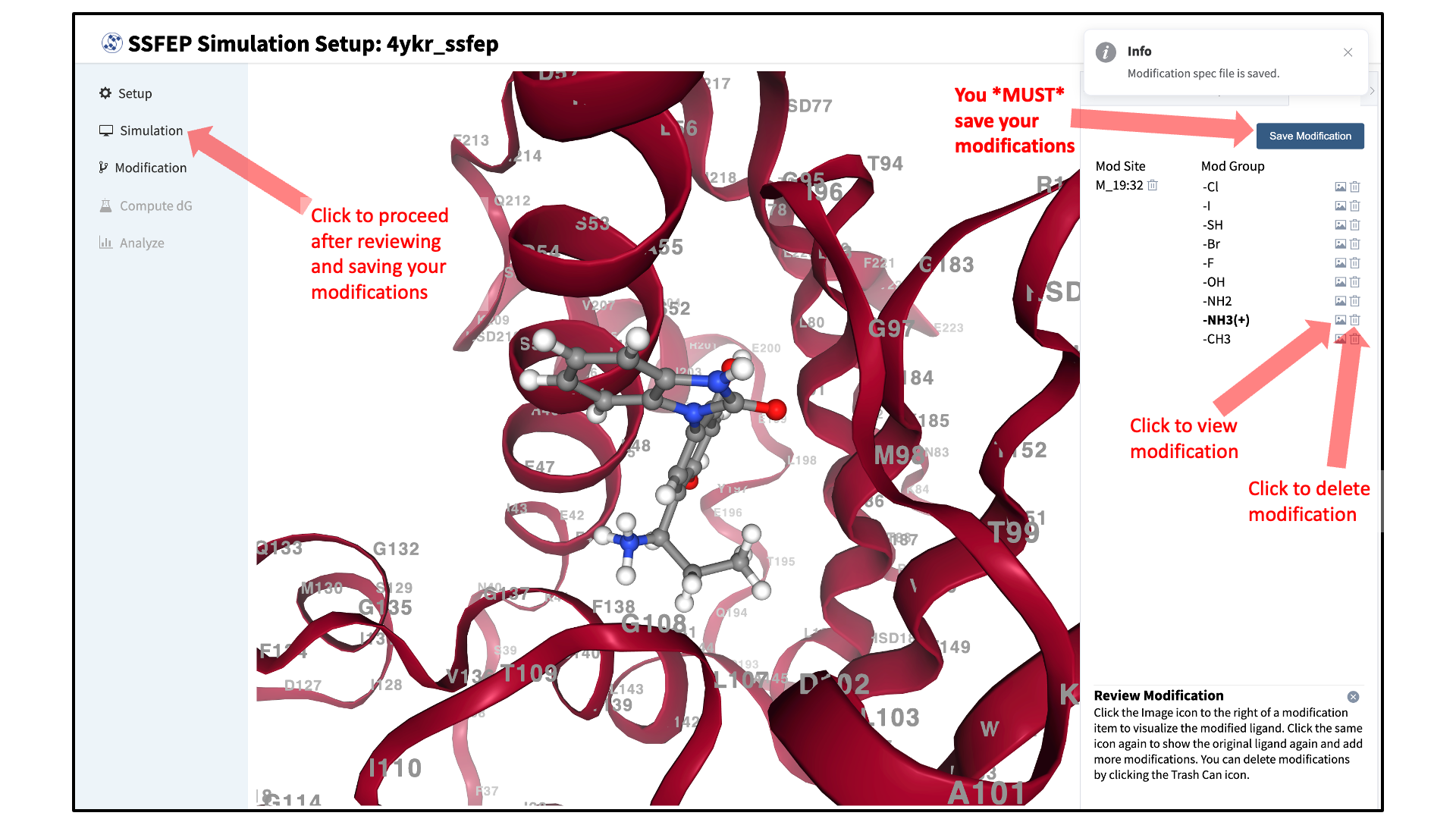
Launch SSFEP simulations:
Your SSFEP simulation can now be started by selecting “Simulation” from the left-hand pane and then clicking the “Run MD Simulation” button in the resulting screen. Before running, you may wish to double check that you have chosen the desired file folder on the remote server and that it has 20+ GB of storage space. There are two parts to SSFEP: a compute-intensive MD simulation and a very rapid \(\Delta \Delta G\) calculation. The compute-intensive MD may take several hours and is done only once. Using the resulting MD data, the rapid \(\Delta \Delta G\) calculation is able to test thousands of functional group modifications to your parent ligand in under an hour. Should you wish to test additional modifications to your parent ligand at a later time in the project, there is no need to re-run the compute-intensive MD, which makes SSFEP a very efficient method.
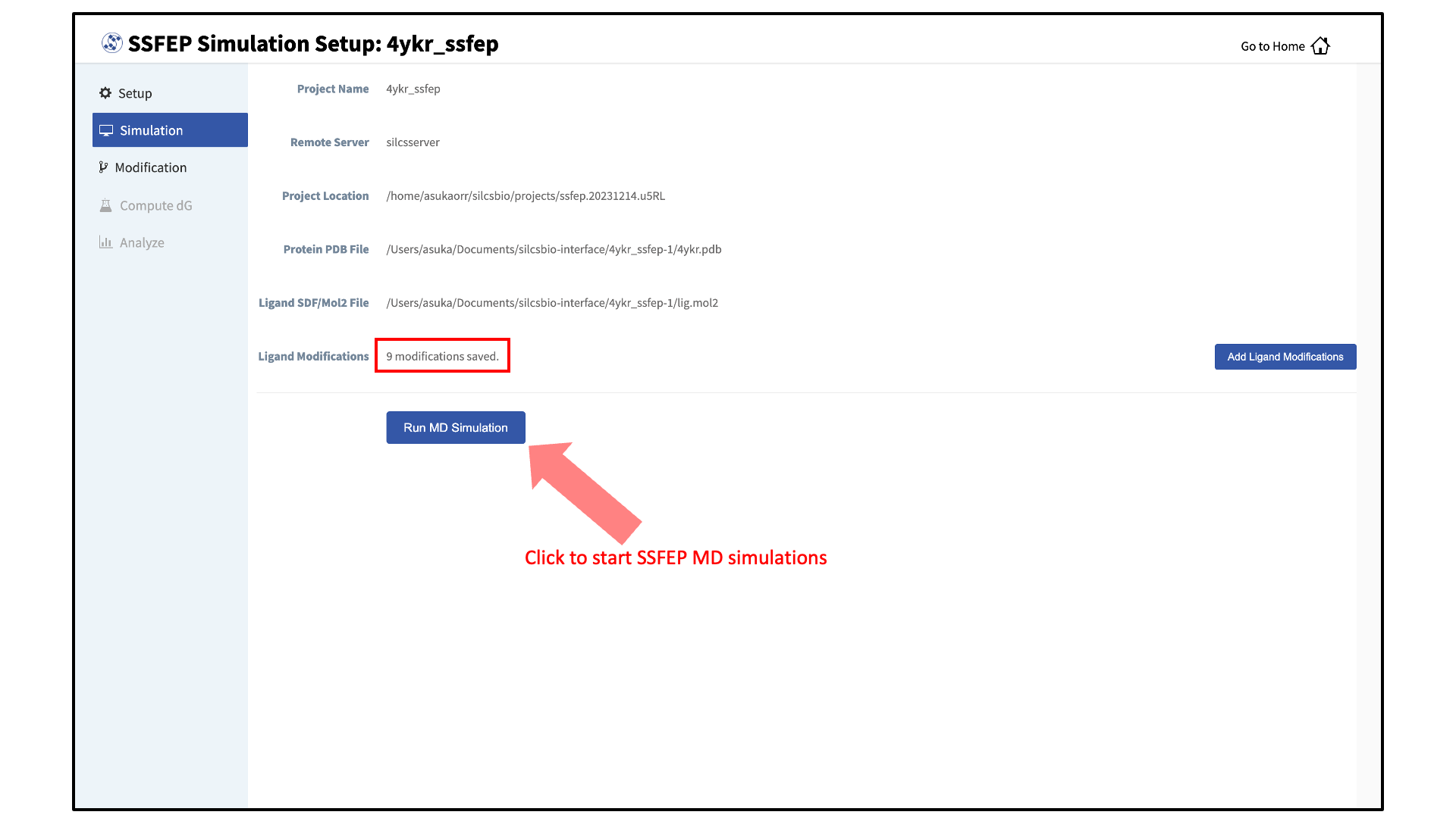
10 compute jobs will be submitted to the queueing system (five for the ligand and five for the protein–ligand complex) on your remote server. Job progress will be displayed in this same window. The status of each job is shown next to its progress bar: “Q” for queued and “R” for running, At this point, your jobs are in progress and you may safely quit the SilcsBio GUI or go back to the Home page to do other tasks.
If a job encounters an error and does not finish, a “restart” button will appear next to the status. If the restart button is used, the job will be resubmitted to the queue and continue from the last cycle of the calculation.
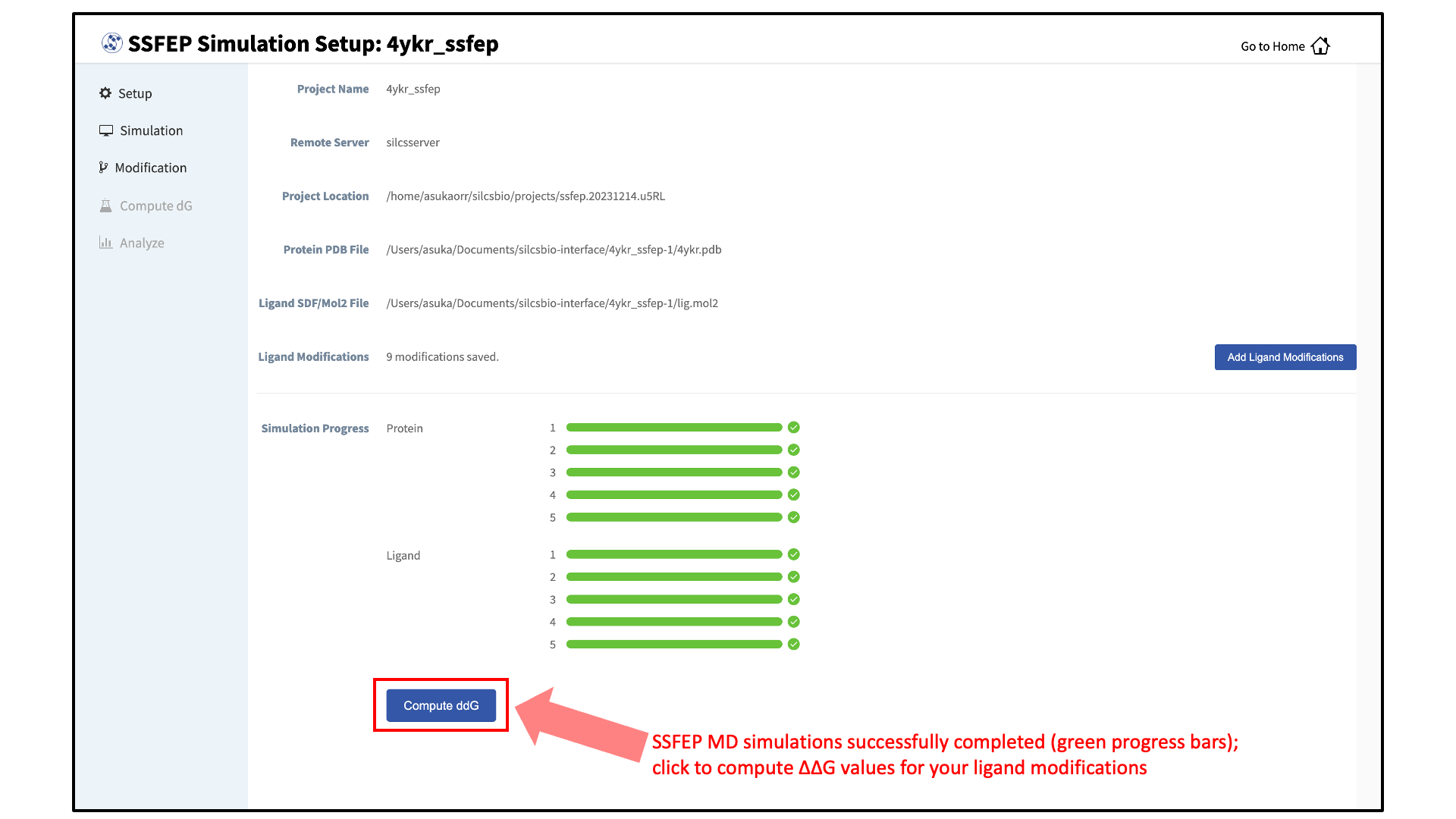
Calculate and collect \(\Delta \Delta G\) values:
Once the MD simulation stage has finished, calculate the \(\Delta \Delta G\) values for your list of modifications by clicking on the “Compute ddG” button at the bottom of the page.
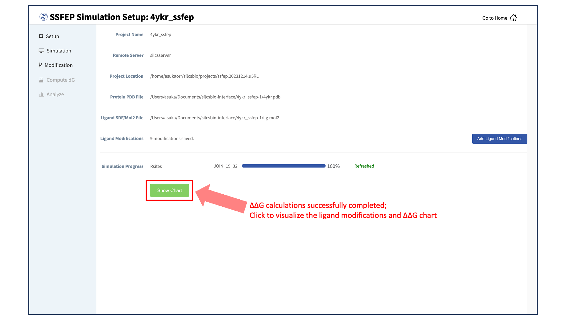
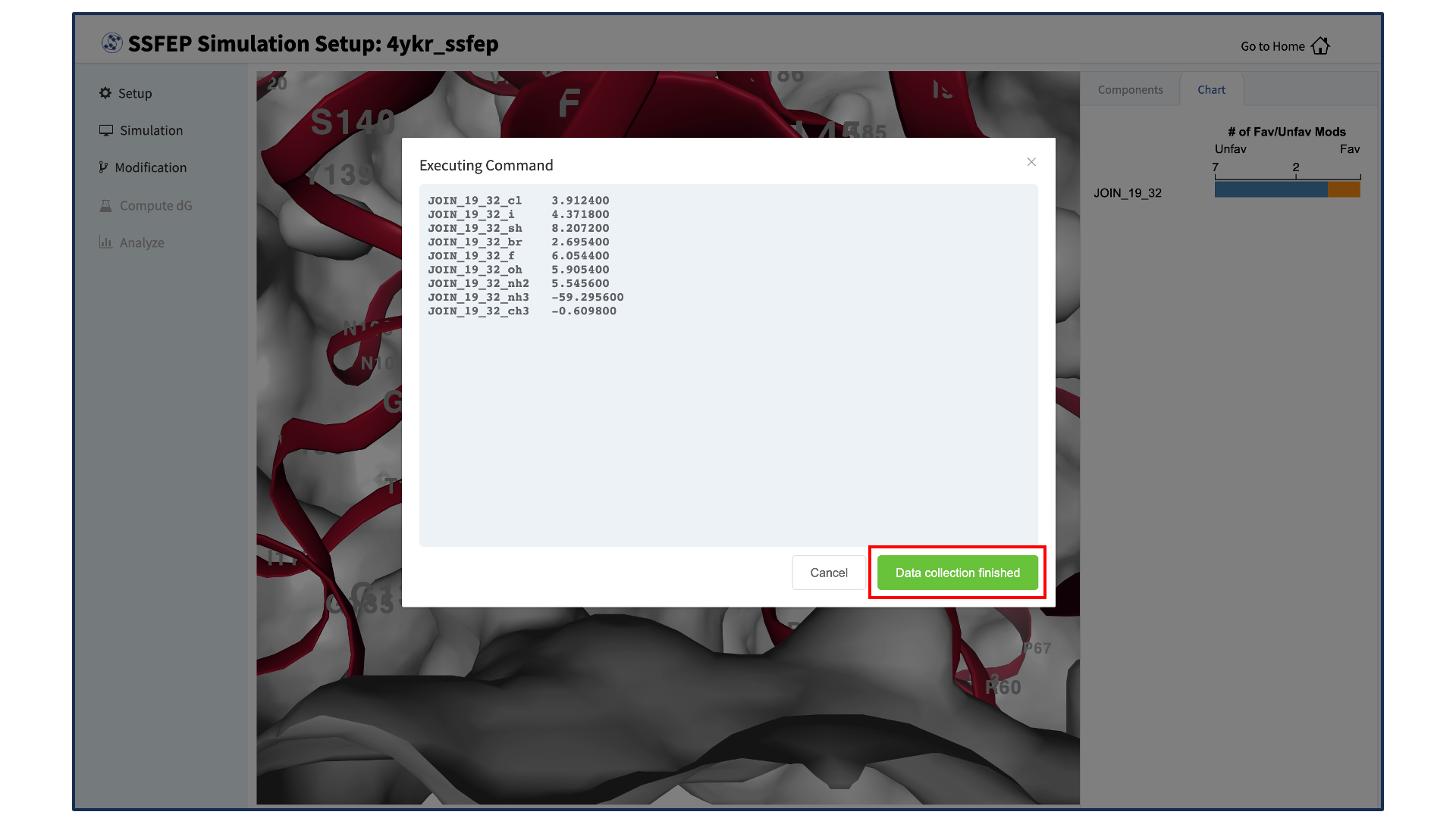
The completion of the \(\Delta \Delta G\) calculations will be indicated by the appearance of the green “Show Chart” button at the bottom of the screen. Click the green “Show Chart” button to collect the data onto the local server. Once data collection is completed, a green “Data collection finished” button will appear. Clike the “Data collection finished” button to proceed.
Visualize \(\Delta \Delta G\) direction:
The predicted changes in direction of binding affinity relative to the parent ligand for each of your selected modifications are plotted to the right of the screen. You can also visualize the modifications in the protein–ligand complex.
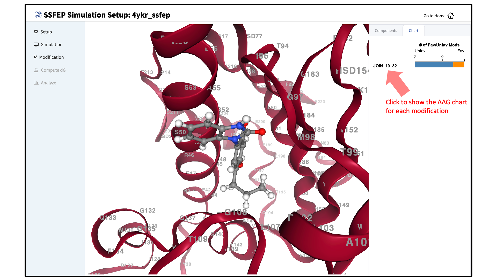
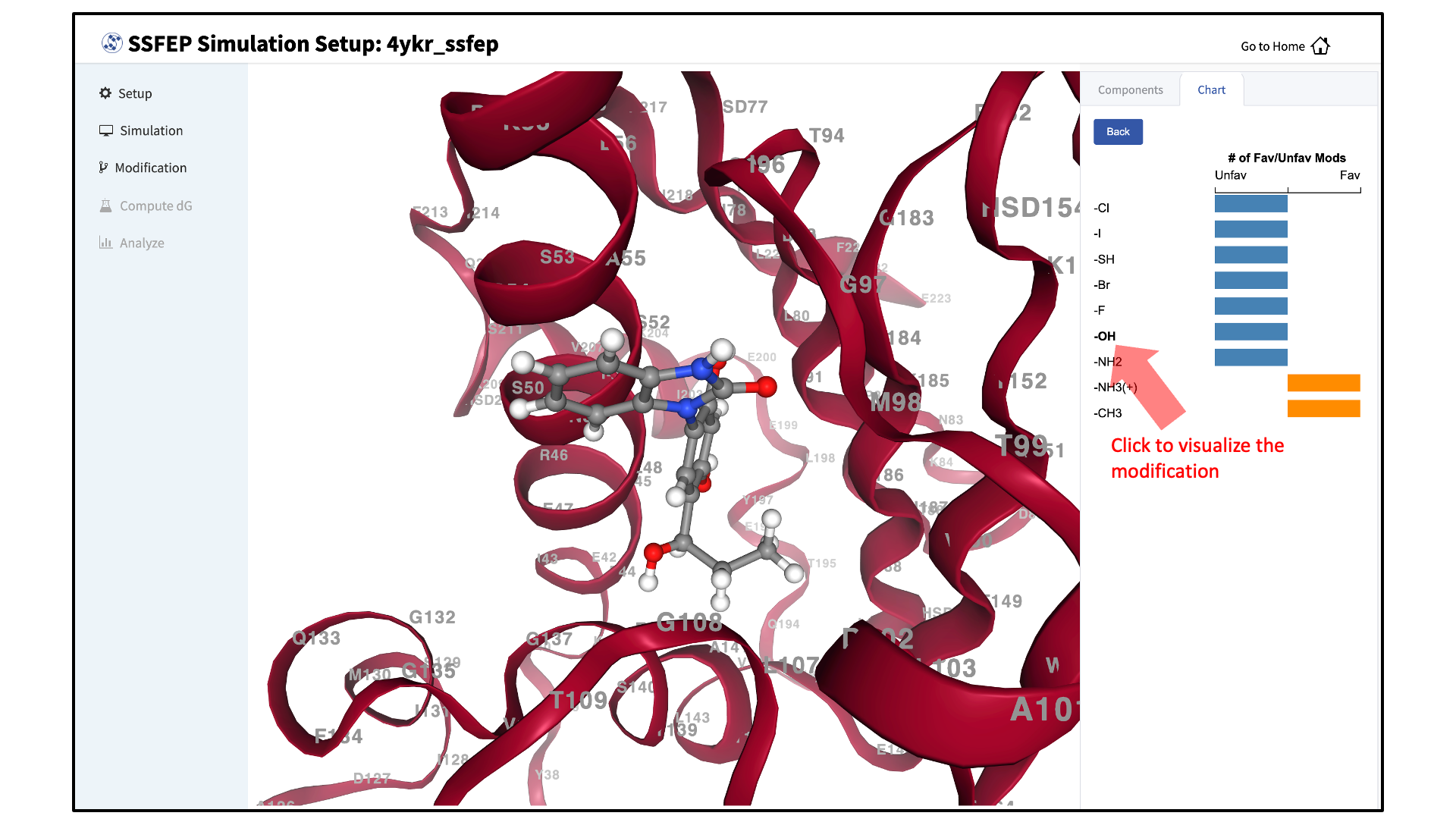
Note
SSFEP is designed to evaluate small modifications, and results are best interpreted qualitatively. Therefore GUI-created charts indicate the predicted change in direction of the binding affinity relative to the parent ligand.
For additional details on SSFEP, please see SSFEP: Single Step Free Energy Perturbation.
Modify Ligand for SSFEP
Given an input parent ligand structure, the SilcsBio GUI provides an intuitive way to modify ligands and save the modified ligand structures in Mol2 format. The resulting structures can be used as input as a parent ligand in the SSFEP Suite. Ligand modifications can be built independently of any other task by choosing Modify ligand for SSFEP from the Home page. For instructions on how to modify ligands, please refer to Ligand Modifications Using the SilcsBio GUI.
CGenFF Suite Quickstart
The CHARMM General Force Field (CGenFF) covers a wide range of chemical groups present in biomolecules and drug-like molecules. The CGenFF program automatically assigns high-quality atom types and parameters to an input molecule in seconds. The resulting topology and parameters are compatible with the CHARMM36 force field, allowing simulations of the target molecule with a vast range of macromolecules, including proteins, lipids, nucleic acids, and carbohydrates, as well as other small molecules. The CGenFF program is available through the SilcsBio GUI under the CGenFF Suite. Additional information on CGenFF and the CGenFF program can be found in Background.
SilcsBio GUI users can access the CGenFF Suite by selecting from the menu bar.

The CGenFF Suite Home page provides easy access for users to
Begin a new CGenFF project (New CGenFF project)
Continue an existing CGenFF project (Continue CGenFF project)
The CGenFF Suite also provides convenient access to general tools under SETUP & GENERAL at the bottom of the page.
For additional information on these tools, please click on their links. Details on how to use the CGenFF program through the SilcsBio GUI are provided below.
CGenFF Parameter Assignment Using the GUI
To begin a new CGenFF project, follow these steps:
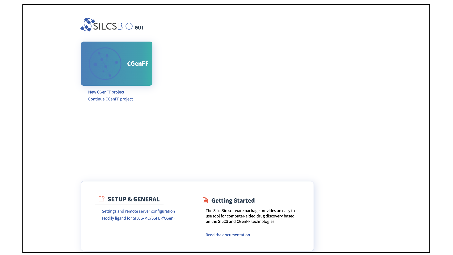
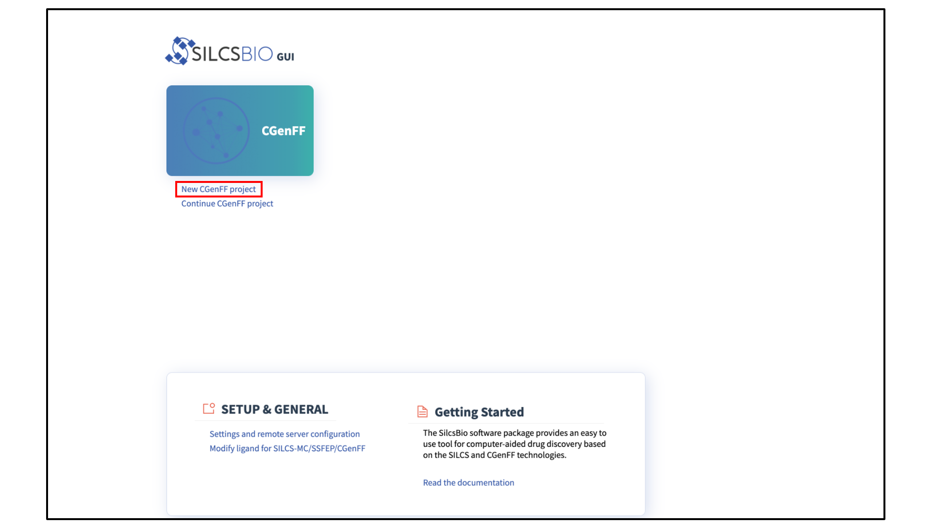
Begin a new CGenFF project:
Select New CGenFF project from the Home page.
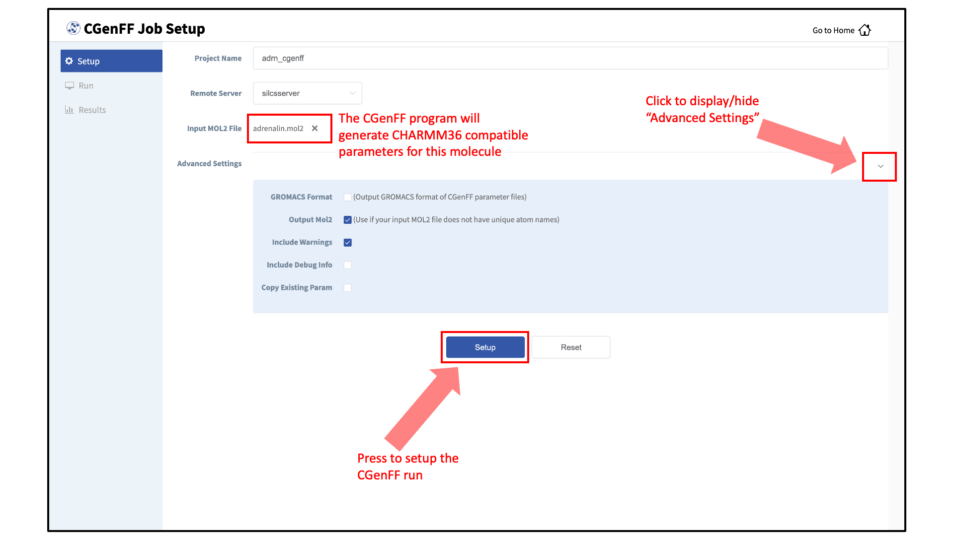
Enter a project name and select the remote server:
Enter a project name and select the remote server where the CGenFF job will run. Input and output files from the CGenFF job will be stored on this server. For information on setting up the remote server, please refer to Remote Server Setup. Next, select a molecule Mol2 file. As described in File and Directory Selection, choose a file from your local computer (“localhost”) or from any server you had configured through the Remote Server Setup process. For correct atom typing, it is important that all hydrogens are present, the system has correct protonation and tautomeric states, and that the bond orders are correct.
Set up the CGenFF job:
Select additional options under “Advanced Settings”:
“GROMACS Format”: The CGenFF assigned parameters, by default, are output in CHARMM compatible format. GROMACS compatible topology and parameter files can be specified by selecting the “GROMACS Format” option.
“Output Mol2”: If your input Mol2 does not have unique atom names, the CGenFF program will rename the atoms and the parameter file will reflect the names of the renamed atoms. In this case, it is advised to select the “Output Mol2” option.
“Include Debug Info”: In the event that the input molecule results in an error, you may select the “Include Debug Info” to identify possible erroneous entries in the input Mol2 file (e.g., missing hydrogen atoms).
“Copy Existing Param”: By default, the CGenFF program will only output newly generated parameters as users are expected to use the force field in conjunction with the CHARMM36 force field. The parameters for which CGenFF directly applies to the input molecule can be explicitly listed in the output parameter file by selecting the “Copy Existing Param” option.
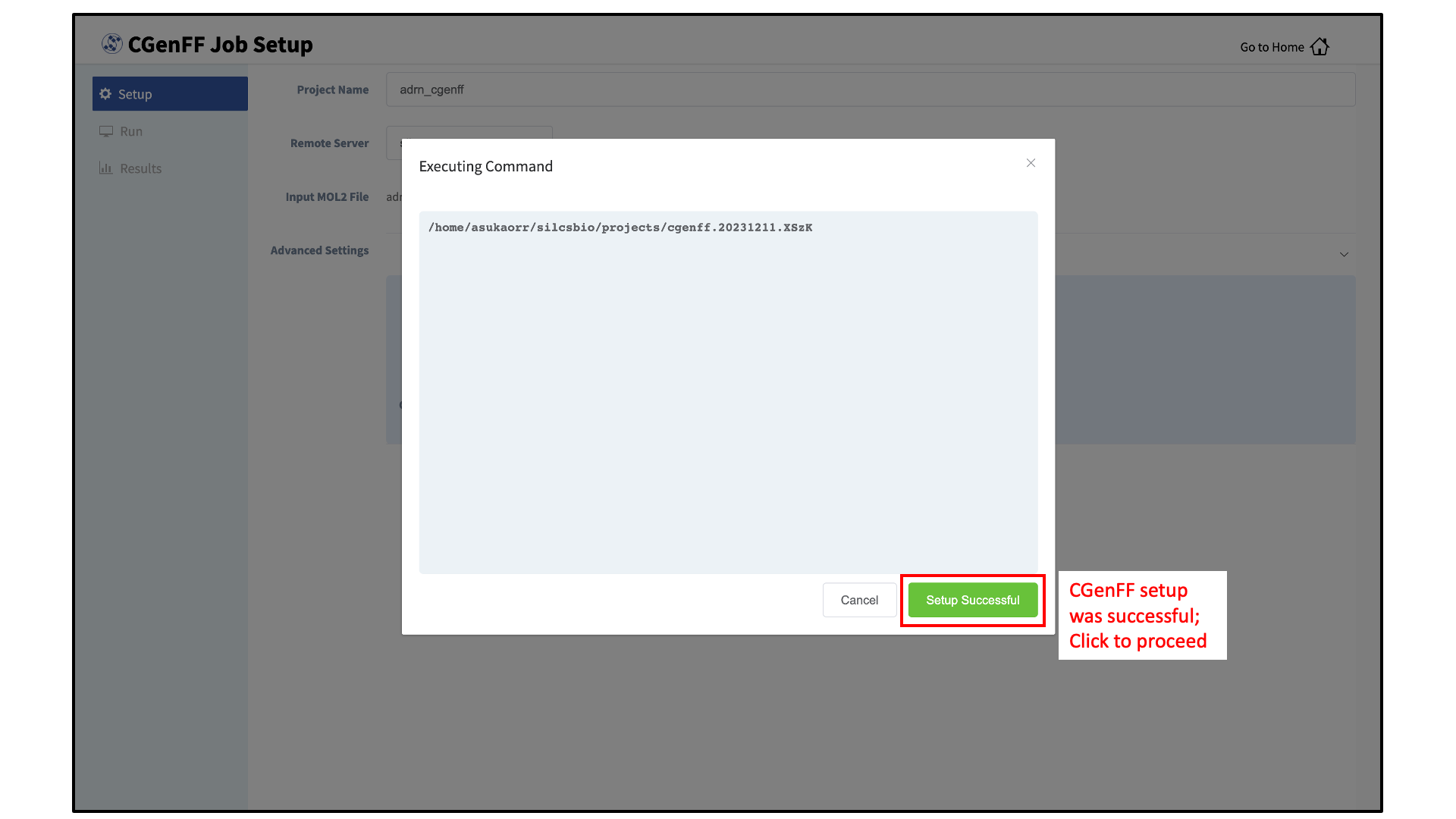
After all information is specified, click the “Setup” button to proceed. Once the CGenFF job is set up, the GUI will indicate that the setup was successful by displaying a green “Setup Successful” button. Click the green “Setup Successful” button to continue.
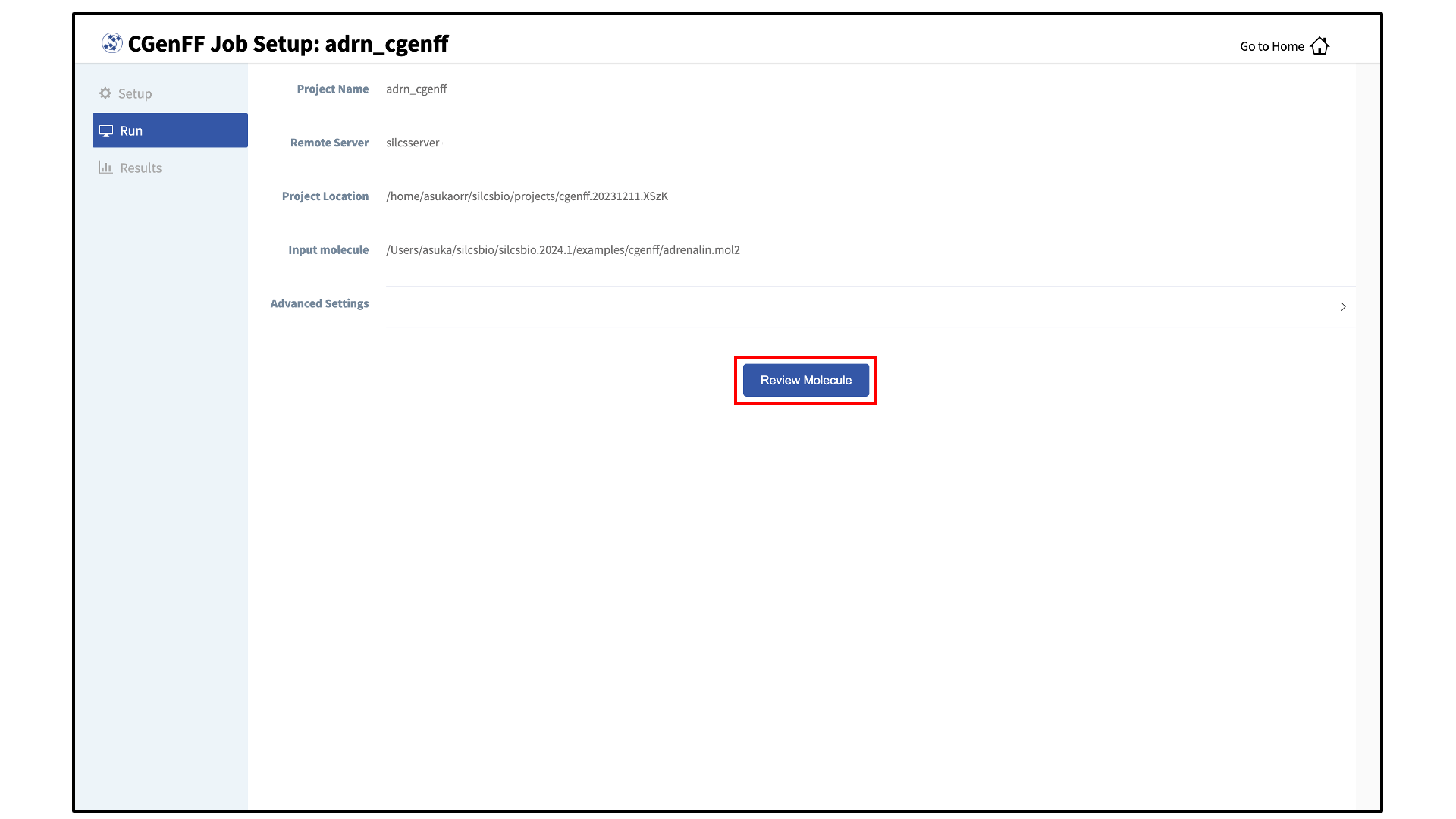
Review the ligand:
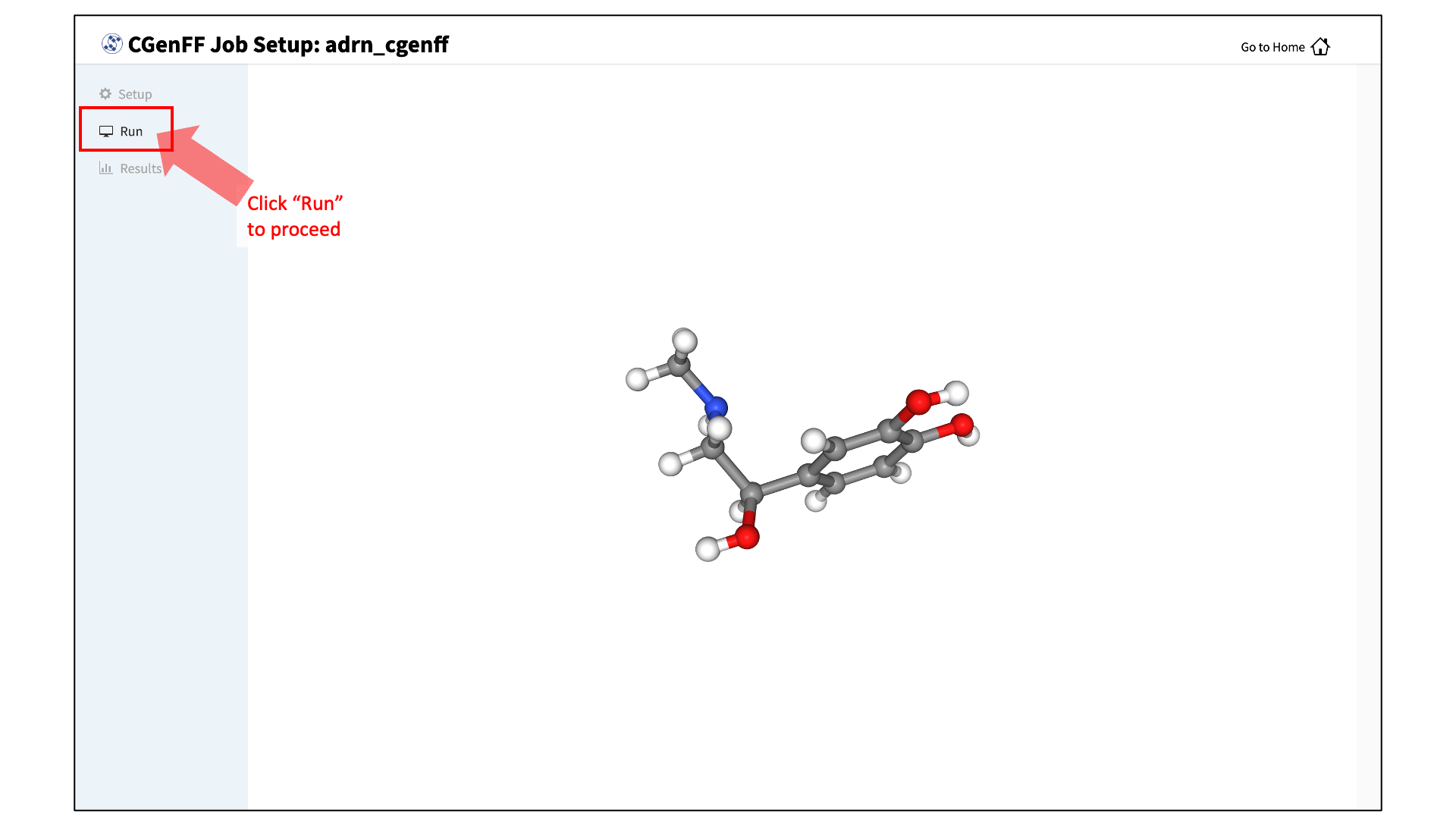
After setting up the CGenFF run, the GUI will prompt you to review your molecule. Click the “Review Molecule” button at the bottom of the screen to visualize the molecule. After reviewing the molecule, click “Run” in the sidebar menu to continue.
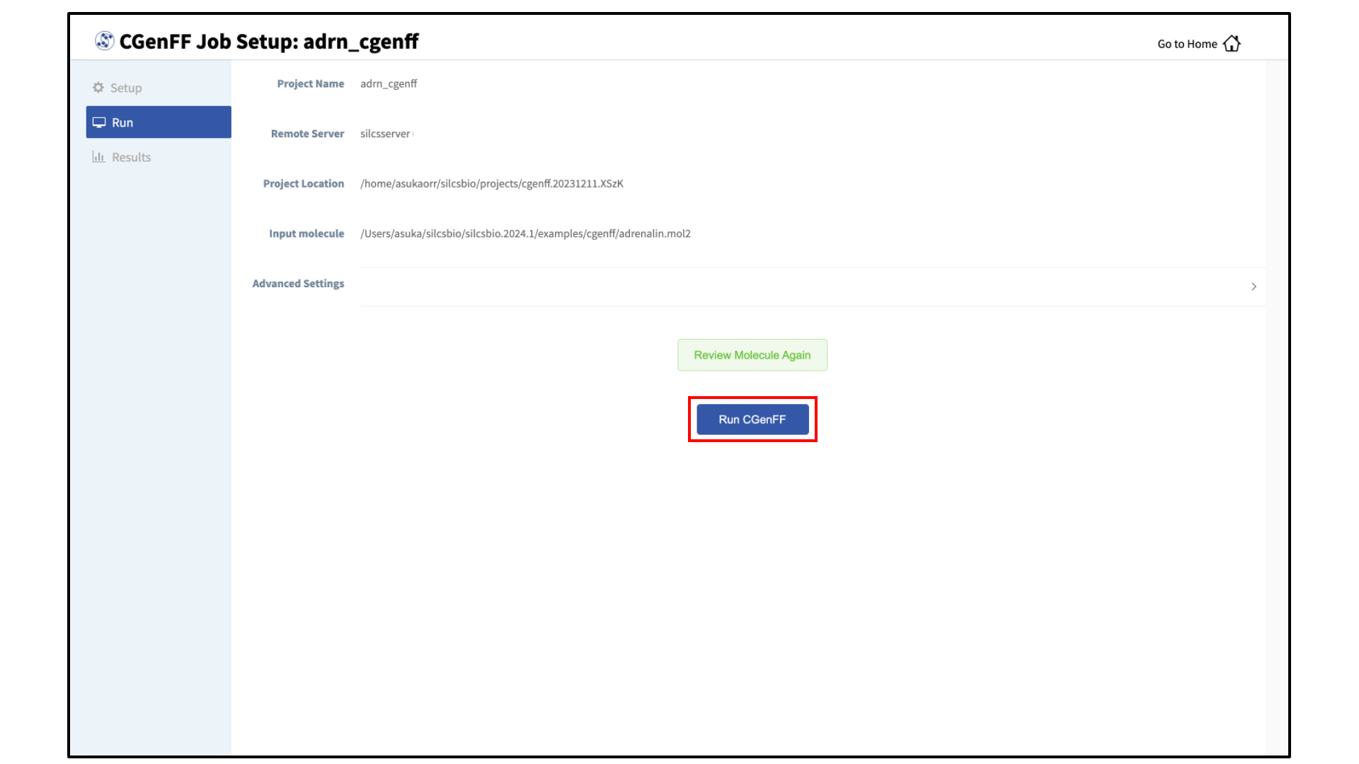
Launch the CGenFF job:
To run the CGenFF program, click the “Run CGenFF” button at the bottom of the page. You may also review the molecule again using the “Review Molecule Again” button.
Download CGenFF assigned topology and parameters:
Once the CGenFF program assigns force field parameters to the molecule, the results will be downloadable by clicking the green “Download Result” button.
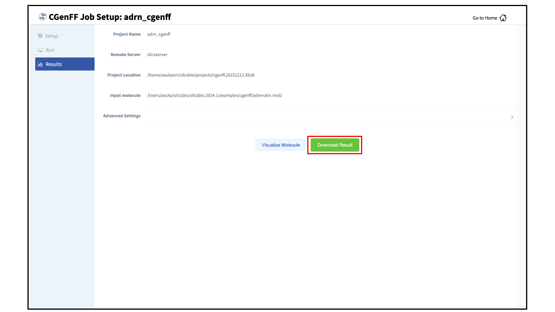
For more information on the output stream file format and advanced CGenFF usage using the CLI, please continue on to CGenFF Using the CLI. Please contact support@silcsbio.com if you need additional assistance.
Modify Ligand for CGenFF
Given an input parent ligand structure, the SilcsBio GUI provides an intuitive way to modify ligands and save the modified ligand structures in Mol2 format. The resulting structures can be used as input to the CGenFF program. Ligand modifications can be built independently of any other task by choosing Modify ligand for CGenFF from the Home page. For instructions on how to modify ligands, please refer to Ligand Modifications Using the SilcsBio GUI.