SILCS Simulations
Background
Fundamental Idea Behind SILCS
The design of small molecules that bind with optimal specificity and affinity to their biological targets, typically proteins, is based on the idea of complementarity between the functional groups in a small molecule and the binding site of the target. Traditional approaches to ligand identification and optimization often employ the one binding site/one ligand approach. While such an approach might be straightforward to implement, it is limited by the resource-intensive nature of screening and evaluating the affinity of large numbers of diverse molecules.
Functional group mapping approaches have emerged as an alternative, in which a series of maps for different classes of functional groups encompass the target surface to define the binding requirements of the target. Using these maps, medicinal chemists can focus their efforts on designing small molecules that best match the maps.
Site Identification by Ligand Competitive Saturation (SILCS) offers rigorous free energy evaluation of functional group affinity pattern for the entire 3D space in and around a macromolecule (globular protein [7], membrane protein, or RNA [14]). The SILCS method yields functional group free energy maps, or FragMaps, which are precomputed and then used to rapidly facilitate ligand design. FragMaps are generated by molecular dynamics (MD) simulations that include macromolecule flexibility and explicit solvent/solute representation, thus providing an accurate, detailed, and comprehensive set of data that can be used in database screening, fragment-based drug design, and lead optimization of small molecules.
In the context of biological therapeutics, the comprehensive nature of the FragMaps is of utility for excipient design as all possible binding sites of all possible excipients and buffers can be identified and quantified.
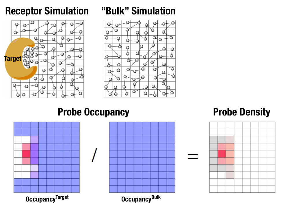
Fig. 1 Illustration of fragment density maps.
Fig. 1 illustrates FragMaps generation. Two MD simulations of a probe molecule (e.g., benzene) are performed in the presence of a protein and in aqueous solution (without protein), resulting in two occupancy maps, \(O^\mathrm{target}\) and \(O^\mathrm{bulk}\), respectively. The GFE (grid free energy) FragMaps are then derived by the following formula [8].
By generating FragMaps using various small solutes (probes) that include a diversity of atoms and chemical functional groups, it is possible to map the functional group affinity pattern of a protein. FragMaps encompass the entire protein such that all FragMap types are in all regions. Thus, information on the affinity of all the different types of functional groups is available in and around the full 3D space of the protein or other target molecule.
A Standard SILCS simulation uses benzene, propane, methanol, imidazole, formamide, dimethylether, methylammonium, acetate, and water as probes to generate Standard SILCS FragMaps. A Halogen SILCS simulation uses fluorobenzene, chlorobenzene, bromobenzene, fluoroethane, chloroethane, and trifluoroethane as probes to generate Halogen SILCS FragMaps. Halogen SILCS FragMaps are used to augment the information provided by Standard SILCS FragMaps.
FragMaps may be used in a qualitative fashion to facilitate ligand design by allowing the medicinal chemist to readily visualize regions where the ligand can be modified or functional groups added to improve affinity and specificity. As the FragMaps include protein flexibility, they indicate regions of the target protein that can “open” thereby identifying regions under the protein surface accessible for ligand binding. In addition to FragMaps, an Exclusion Map is generated based on regions of the system that are not sampled at all by any probe molecules, including water, during the MD simulations. Therefore, the Exclusion Map represents a strictly inaccessible surface.
Many proteins contain binding sites that are partially or totally inaccessible to the surrounding solvent environment that may require partial unfolding of the protein for ligand binding to occur. SILCS sampling of such deep or inaccessible pockets is facilitated by the use of a Grand Canonical Monte Carlo (GCMC) sampling technique in conjunction with MD simulations [10]. Thus, the SILCS technology is especially well-suited for targeting the deep or seemingly inaccessible binding sites found in targets like GPCRs and nuclear receptors.
Once a set of ligand-independent SILCS FragMaps are produced, they can be used for various purposes that rapidly rank ligand binding in a highly computationally efficient manner for multiple ligands WITHOUT recalculating the FragMaps. Applications of SILCS methodology include:
Binding site identification
Binding pocket searching with known ligands
Binding pocket identification via pharmacophore generation
Binding pocket identification via fragment screening
Database screening
SILCS 3D pharmacophore models
Ligand posing using available techniques (Catalyst, etc)
Ligand ranking
Fragment-based ligand design
Identification of fragment binding sites
Estimation of ligand affinity following fragment linking
Expansion of fragment types
Ligand optimization
Qualitative ligand optimization by FragMaps visualization
Quantitative evaluation of ligand atom contributions to binding
Quantitative estimation of relative ligand affinities
Quantitative estimation of large numbers of ligand chemical transformations
SILCS generates 3D maps of interaction patterns of functional group with your target molecule, called FragMaps. This unique approach simultaneously uses multiple different small solutes with various functional groups in explicit solvent MD simulations that include target flexibility to yield 3D FragMaps that encompass the delicate balance of target-functional group interactions, target desolvation, functional group desolvation and target flexibility. The FragMaps may then be used to both qualitatively direct ligand design and quantitatively to rapidly evaluate the relative affinities of large numbers of ligands following the precomputation of the FragMaps.
This chapter goes over the workflow for generating SILCS FragMaps.
FragMap names and underlying probe atoms
Each FragMap generated from a SILCS simulation is the result of computing occupancies for one or more kinds of atoms associated with the SILCS probes. The tables below provide the complete lists for Standard SILCS and for Halogen SILCS simulations.
FragMap name |
generated from probe atom(s) |
|---|---|
acec |
acetate carboxylate carbon |
apolar |
generic apolar carbons (benc+prpc) |
benc |
benzene carbons |
dmeo |
dimethyl ether oxygen |
forn |
formamide nitrogen |
foro |
formamide oxygen |
hbacc |
generic hydrogen bond acceptors (foro+dmeo+imin) |
hbdon |
generic hydrogen bond donors (forn+iminh) |
imin |
imidizole nitrogen (h-bond acceptor) |
iminh |
imidizole nitrogen (h-bond donor) |
mamn |
methylamine nitrogen |
meoo |
methanol oxygen |
prpc |
propane carbon |
tipo |
water oxygen |
FragMap name |
generated from probe atom |
|---|---|
brbx |
bromobenzene bromine |
clbx |
chlorobenzene chlorine |
clex |
chloroethane chlorine |
fetx |
fluoroethane fluorine |
flbc |
fluorbenzene fluorine |
tfec |
trifluoroethane carbon bonded to fluorines |
The FragMap with the name “excl” is a special case. It is the SILCS Exclusion Map, and it enumerates all voxels where no probe molecule (including water) sampling occurred.
For Globular Proteins
SILCS Simulations Using the SilcsBio GUI
Please see SILCS Simulations Using the GUI as described in Graphical User Interface (GUI) Quickstart for a step-by-step description for using the SilcsBio GUI for SILCS simulations.
FragMap generation using SILCS begins with a well-curated protein structure file (without ligand) in PDB file format. We recommend keeping only those protein chains that are necessary for the simulation, removing all unnecessary ligands, renaming non-standard residues, filling in missing atomic positions, and, if desired, modeling in missing loops. Please contact support@silcsbio.com if you need assistance with protein preparation.
A typical SILCS simulation can produce output totaling in excess of 100 GB, so please select a “Project Directory” folder on your server with appropriate free space. The default is determined by the “Project Directory” setting during Remote Server Setup.
The setup process automatically builds the topology of the simulation system, creating metal-protein bonds if metal ions are present, rotates side chain orientations to enhance sampling, and places probe molecules around the protein. If missing loops were not modeled into the input PDB file, the amino acids on either side of each missing loop will be automatically capped with neutral functional groups.
Tip
For users with access to both the SILCS-Small Molecule Suite and the CGenFF Suite, running standard MD simulation can be helpful to determine the stability of or refine the protein structure to be used as an initial structure for SILCS simulations. Specifically, this may be very helpful if the user has obtained the protein structure from homology modeling or alphafold. For more information on standard MD simulations with the CGenFF Suite, please refer to Standard Molecular Dynamics (MD) Simulations.
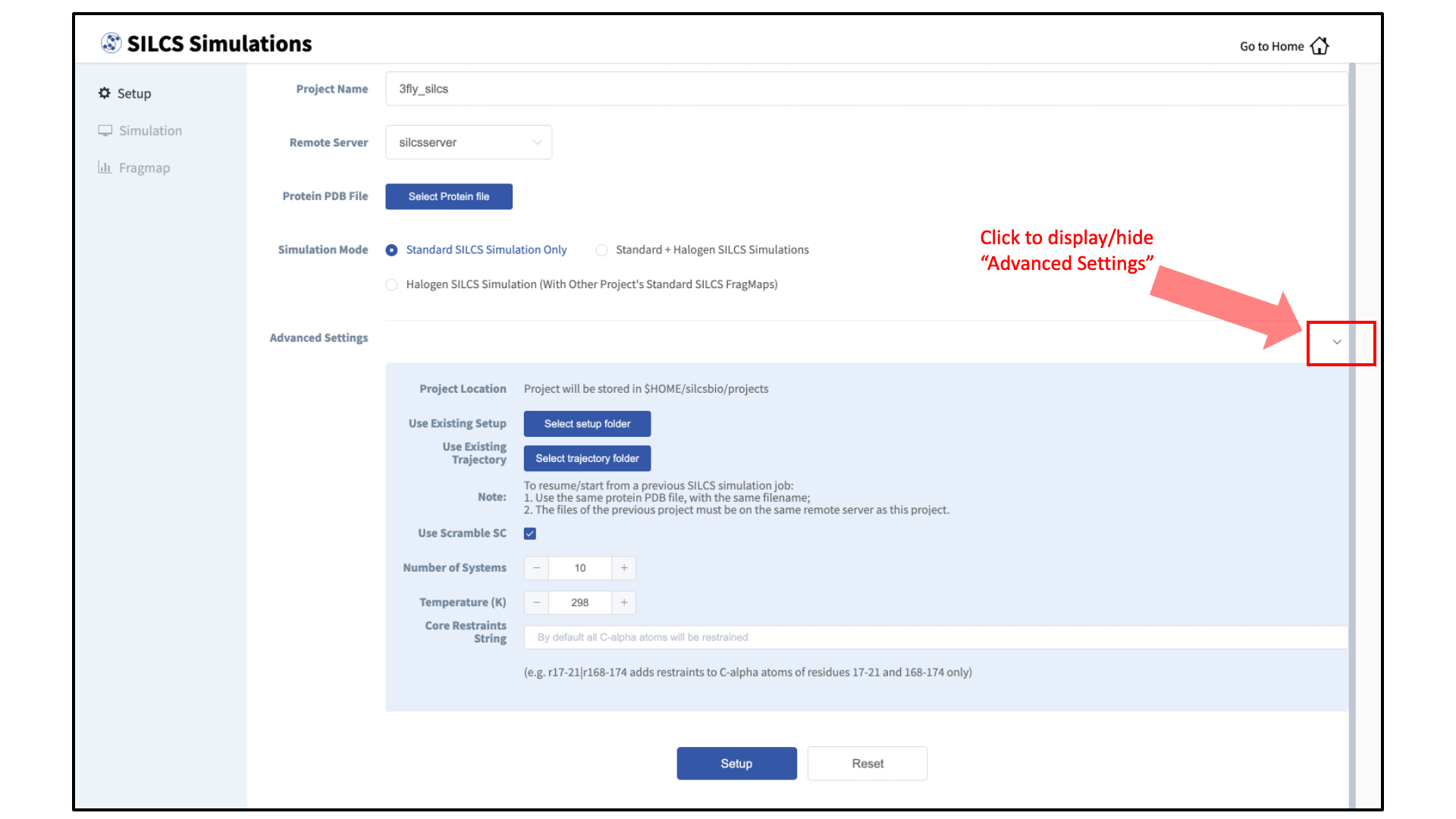
During setup, you will need to decide whether to run a Standard SILCS Simulation, Standard + Halogen SILCS Simulations, or a Halogen SILCS Simulation (with another project’s Standard SILCS FragMaps). All functionality in the SILCS platform requires FragMaps from a Standard SILCS Simulation. FragMaps from Halogen SILCS Simulations can supplement Standard SILCS FragMaps for SILCS-MC: Ligand Optimization and for SILCS-MC: Docking and Pose Refinement. Visualization of Halogen SILCS FragMaps can be very useful for qualitatively informing ligand design (see Visualizing SILCS FragMaps). See FragMap names and underlying probe atoms for a complete listing of both Standard and Halogens SILCS probe molecules and the resulting FragMaps.
Note
Running a Halogen SILCS simulation requires the same computation time as running a Standard SILCS simulation, so selecting “Standard + Halogen SILCS Simulations” will consume double the computational resources as selecting “Standard SILCS Simulation”. The default is to generate and run 10 systems each for a Standard SILCS simulation and for a Halogen SILCS simulation. Therefore, if your computing resource has 10 nodes, it will take twice as much wall time to complete a “Standard + Halogen SILCS Simulations” job as to complete a “Standard SILCS Simulation”. However, if you have access to 20 nodes simultaneously, the wall time will be the same, since each individual system is run independently of the others.
While the same identical input protein coordinates are used for constructing each of these systems, each system is unique because the probe molecules are randomly placed. Additional diversity is added by default to initial coordinates by scrambling the sidechains of exposed amino acids.
Tip
Advanced Settings options during setup allow you to change the scrambling of sidechains (default: on), the number of systems (default: 10), the simulation temperature (default 298 K), and which residues are subjected to restraints on C-alpha atoms (default: all residues). We STRONGLY urge you to use these default settings, which have been selected based on extensive experience.
It is also possible to choose an existing setup folder or an existing trajectory folder at this time.
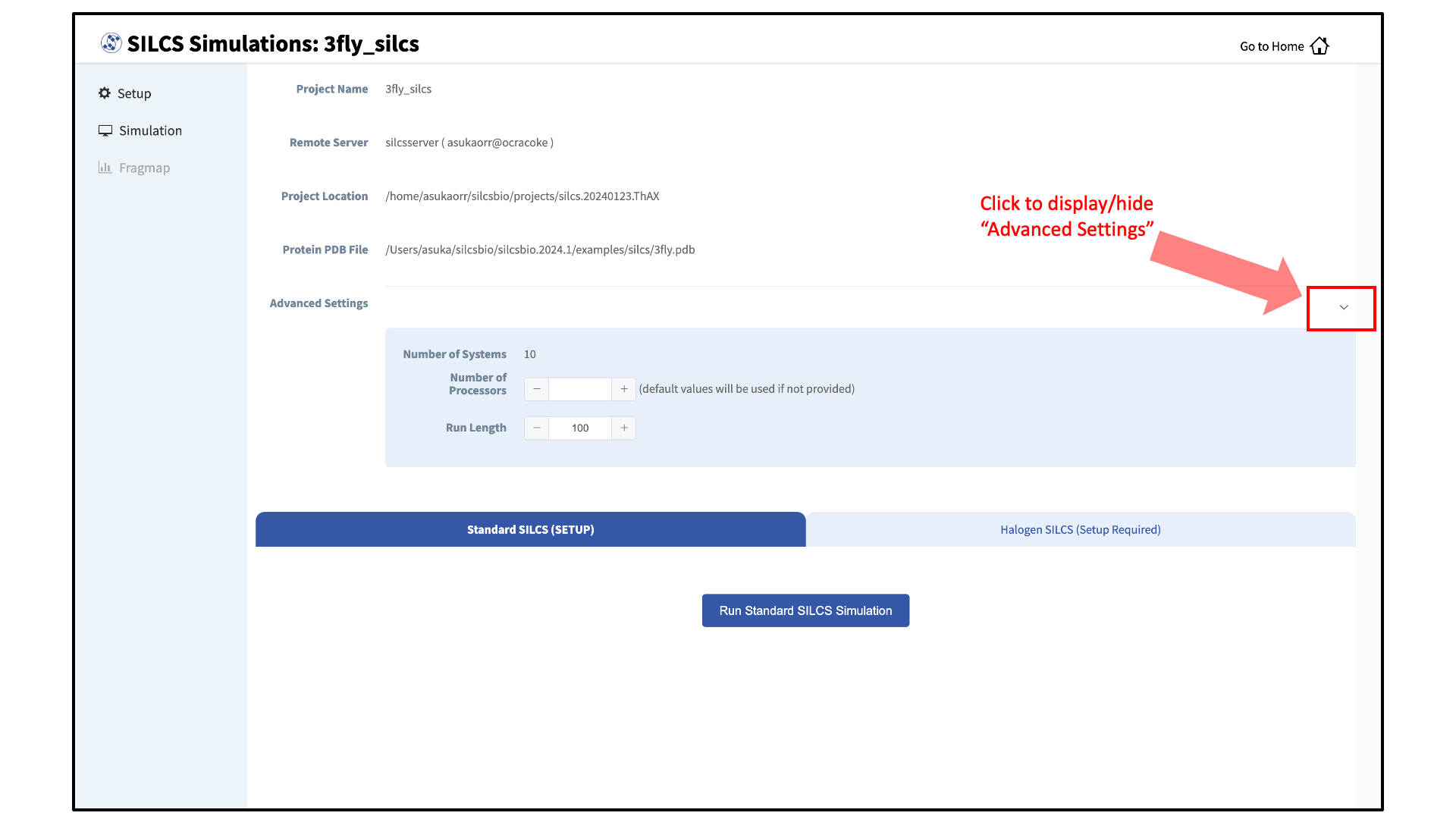
Once the systems are set up, you will need to start the SILCS simulations. There are separate tabs for running the Standard SILCS simulation and the Halogen SILCS simulation, and you will need to use each tab and the “Run…” button underneath that tab to run the corresponding simulation type.
Tip
Advanced Settings options allow you to change the number of systems that are run, as well as the number of processors used for each run and the length of each run. Leaving these fields blank will result in default values being used. We STRONGLY urge you to use the default settings. If you have concerns about the number of processors per run, please contact your system administrator.
Tip
If a simulation stops prematurely, the progress bar will turn red and show a “Restart” option. When the job is restarted, completed cycles will be automatically skipped and the progress will update to where the job had stopped. That is to say, restarting a failed or stopped job will not cause you to lose existing job progress.
SILCS Simulations Using the CLI
Please see SILCS Simulations Using the CLI as described in Command Line Interface (CLI) Quickstart for a step-by-step description for using the Command Line Interface (CLI) for SILCS simulations. This section covers additional parameters and options that may be included in your SILCS simulations.
FragMap generation using SILCS begins with a well-curated protein structure file (without ligand) in PDB file format. We recommend keeping only those protein chains that are necessary for the simulation, removing all unnecessary ligands, renaming non-standard residues, filling in missing atomic positions, and, if desired, modeling in missing loops. Please contact support@silcsbio.com if you need assistance with protein preparation.
Set up the SILCS simulations:
${SILCSBIODIR}/silcs/1_setup_silcs_boxes prot=<Protein PDB>Warning
The setup program internally uses the GROMACS utility
pdb2gmx, which may have problems processing the protein PDB file. The most common reasons for errors at this stage involve mismatches between the expected residue name/atom names in the input PDB and those defined in the CHARMM force-field.To fix this problem: Run the
pdb2gmxcommand manually from within the1_setupdirectory for a detailed error message. The setup script already prints out the exact commands you need to run to see this message.cd 1_setup pdb2gmx –f <PROT PDB NAME>_4pdb2gmx.pdb –ff charmm36 –water tip3p –o test.pdb –p test.top -ter -merge allOnce all the errors in the input PDB are corrected, rerun the setup script.
The setup command offers a number of options. The full list of options can be reviewed by simply entering the command without any input.
Required parameter:
Path and name of the input protein PDB file:
prot=<protein PDB file>Tip
For users with access to both the SILCS-Small Molecule Suite and the CGenFF Suite, running standard MD simulation can be helpful to determine the stability of or refine the protein structure to be used as an initial structure for SILCS simulations. Specifically, this may be very helpful if the user has obtained the protein structure from homology modeling or alphafold. For more information on standard MD simulations with the CGenFF Suite, please refer to Standard Molecular Dynamics (MD) Simulations.
Optional parameters:
Number of independent simulation systems:
numsys=<# of simulations; default=10>SILCS simulations, by default, consist of 10 replicate simulations, each with different initial velocities, to enhance sampling. The number of simulations can be adjusted using the
numsyskeyword.Skip the
pdb2gmxGROMACS utility:skip_pdb2gmx=<true/false; default=false>Path and name of bound cofactor Mol2:
lig=<lig.mol2; default=empty/NULL>If the input structure contains a cofactor and you wish to compute your FragMaps in the presence of the cofactor, remove the cofactor from the input PDB file and provide a separate Mol2 file of the cofactor in the correct position and orientation with respect to the target protein. Provide the path and name of the cofactor Mol2 file using the
ligkeywordNote
If your input structure contains a metal ion, please see What happens when I set up SILCS simulations with an input structure containing a metal ion?
Application of weak harmonic positional restraints:
core_restraints_string=<restrained residues, e.g., "r 17-21 | r 168-174"; default=empty/NULL>By default, a weak harmonic positional restraint, with a force constant of ~0.1 kcal/mol/Å2, is applied to all C-alpha atoms during SILCS simulations. This option lets you modify this default.
For example, if
core_restraints_string="r 17-160 | r 168-174"is supplied, then only the C-alpha atoms in residues 17 to 160 and residues 168 to 174 will be restrained.Re-orientation of residue side chains:
scramblesc=<true/false; default=true>When set to
truethescramblesckeyword re-orients the side chain dihedrals of the protein residues.Simulation box size:
margin=<system margin (Å); default=15>By default, the simulation system size is determined by adding a 15 Å margin to the size of the input protein structure. The size of the simulation box can be customized by using the
marginkeyword.SILCS probes with halogen-containing functional groups:
halogen=<true/false; default=false>SILCS simulations can be performed with SILCS probes that contain halogen-containing functional groups by including
halogen=truein the commandline. See Setup with halogen probes for more details.
Submit the SILCS GCMC/MD jobs to the queue:
Following completion of the setup, run 10 GCMC/MD jobs using the following script:
${SILCSBIODIR}/silcs/2a_run_gcmd prot=<Protein PDB>This script will submit 10 jobs to the predefined queue. Each job runs out 100 ns of GCMC/MD with the protein and the solute molecules.
This command offers a number of options. The full list of options can be reviewed by simply entering the command without any input.
Required parameter:
Path and name of the input protein PDB file:
prot=<protein PDB file>
Optional parameters:
Simulation temperature:
temp=<simulation temperature; default=298>
The input simulation temperature should be entered in Kelvin units. By default, the temperature is set to 298 K.
Number of cores per simulation:
nproc=<# of cores per simulation; default=8>
Generate input files without submitting jobs to the queue:
batch<only generate inputs and not submit jobs true/false; default=false>
Use halogen probes:
halogen=<use halogen probes; true/false; default=false>
The SILCS simulation will be performed with halogen probes when
halogen=true. For more information, please refer to Setup with halogen probes.
Tip
SILCS simulations are run at a temperature of 298 K by default, and most published work with SILCS has used this default temperature. It is possible to set a custom temperature by adding the
temp=<simulation temperature; default=298>option to the2a_run_gcmdcommand. For example,temp=310would run the SILCS simulations at 310 K, which may enhance protein conformational sampling.Once the simulations are complete, the
2a_run_gcmd/[1-10]directories will contain*.prod.100.rec.xtctrajectory files. If these files are not generated, then your simulations are either still running or stopped due to a problem. Look in the log files within these directories to diagnose problems.To check job progress, use the following command:
${SILCSBIODIR}/silcs/check_progressThis will provide a summary list of the SILCS jobs consisting of the job path, the job number, the task ID, the job status, and the current/total number of GCMC/MD cycles. Job status values are: Q [queued], R [running], E [successfully ended], F [failed], NA [not submitted].
Generate FragMaps:
Once your simulations are done, generate the FragMaps using the following command:
${SILCSBIODIR}/silcs/2b_gen_maps prot=<Protein PDB>Required parameter:
Path and name of the input protein PDB file:
prot=<protein PDB file>
Optional parameters:
Simulation box size:
margin=<size of margin in the map; default=10>
Generate halogen maps:
halogen=<true/false; default=false>
If the SILCS simulations were performed with halogen probes, then use
halogen=true. For more information, please refer to Setup with halogen probes.Reference structure:
ref=<reference PDB; default=same PDB file given in prot>
By default, the FragMaps will be oriented around the protein structure that was used as the initial structure for the SILCS simulations. The FragMaps can also be oriented around a different structure by specifying it with
ref=.Generate protein side chain maps:
protmap=<true/false; generate protein side chain maps; default=true>
The probability distribution of protein side chains can also be calculated and stored in protein side chain maps. When
protmap=true, this information will be calculated and stored.Spacing between voxels:
spacing=<map spacing; default=1.0>
The probabiliy of each functional group occupying a voxel is used to calculate GFE values. By default, the spacing between each voxel is 1.0 Å.
First cycle number to use for map generation:
begin=<cycle number to begin for map generation; default=1>
Last cycle number to use for map generation:
end=<cycle number to end for map generation; default=100>
Collect and merge trajectory:
traj=<collect and merge protein trajectory; default=false>
Specification that v2023.x or older was used for
2a_run_gcmd:oldversion=<true if v2023.x or older versions used to run 2a_run_gcmd step and if traj=true; default=false>
Rewrite
.xtcfiles acording to selection:rewritextc=<input file for gmx make_ndx to rewrite 2a_run_gcmd/*/*nowat.xtc files with new selection; default=empty/NULL>
The above command will submit 10 single-core jobs that will build occupancy maps (FragMaps) spanning the simulation box for select probe molecule atoms representing different functional groups. For a ~50K atom simulation system, this step takes approximately 10-20 minutes to complete. The FragMaps have a default grid spacing of 1 Å.
The next step is to combine the occupancy FragMaps generated from individual simulations and convert them into GFE FragMaps. Each voxel in a GFE FragMap contains a Grid Free Energy (GFE) value for the probe type that was used to create the corresponding occupancy FragMap.
${SILCSBIODIR}/silcs/2c_fragmap prot=<Protein PDB>Required parameter:
Path and name of the input protein PDB file:
prot=<protein PDB file>
Optional parameters:
Generate protein side chain maps:
protmap=<true/false; generate protein side chain maps; default=true>
The probability distribution of protein side chains can also be calculated and stored in protein side chain maps. When
protmap=true, this information will be calculated and stored.Skip overlap coefficient calculation:
skipoc=<true/false; skip overlap coefficient calculation; default=false>
Generate halogen maps:
halogen=<true/false; default=false>
If the SILCS simulations were performed with halogen probes, then use
halogen=true. For more information, please refer to Setup with halogen probes.Generate maps in CNS format:
cns=<true/false; generate maps in CNS format; default=false>
First cycle number to use for map generation:
begin=<cycle number to begin for map generation; default=1>
Last cycle number to use for map generation:
end=<cycle number to end for map generation; default=100>
GFE FragMaps will be created in the
silcs_fragmap_<protein PDB>/mapsdirectory, and PyMOL and VMD scripts to load these file will be created in thesilcs_fragmap_<protein PDB>directory.Additionally, the convergence of the SILCS simulations will be assessed by calculating the overlap coefficient between the occupancy maps generated from the first and second halves of the runs. The output is written to the
overlap_coeff.datfile.Cleanup:
Raw trajectory output files are large. To reduce disk usage due to these files, use the cleanup command:
${SILCSBIODIR}/silcs/2d_cleanup prot=<Protein PDB>Required parameter:
Path and name of input protein PDB file:
prot=<protein PDB file>
Optional parameters:
Number of simulation systems:
numsys=<# of simulations; default=10>
Specification that halogen probes were used in
2a_run_gcmd:halogen=<true/false; default=false>
Delete original files:
delete=<delete original files after tar-balls are created true/false; default=false>
The
2d_cleanupcommand deletes unnecessary files, such as those from the equilibration phase, and deletes hydrogen atoms from production trajectory files for each run directory,1/,2/, etc. It then creates a.tar.gzfile of that directory. That is to say, the contents of1.tar.gzand1/after running cleanup are identical. You may choose to remove either one of those without loss of information, though we strongly recommend comparing the output oftar tvzf <run>.tar.gzwith the output offind <run> -type f, where you replace<run>with1,2, etc. and confirm the contents are identical before deleting anything.
Setup with halogen probes
SILCS probes with halogen-containing functional groups can be useful for extending the diversity of chemical space covered by FragMaps. While a common approach is to consider halogen atoms as non-polar groups, research on non-covalent “halogen bonding” suggests halogen atoms warrant special treatment.
The CHARMM General Force Field CGenFF v.2.3.0+ allows halogen atoms to be treated with lonepairs to achieve directionality in polar interactions. These force field improvements are included in SILCS simulations from version 2020.1 of the SilcsBio software. Halogen-protein interactions are determined using a set of halogenated probes in SILCS simulations: chlorobenzene, fluorobenzene, bromobenzene, chloroethane, fluoroethane, and trifluoroethane.
To use these halogenated SILCS probes in your simulation instead of the
standard SILCS probes, add the halogen=true keyword:
${SILCSBIODIR}/silcs/1_setup_silcs_boxes prot=<Protein PDB> halogen=true
${SILCSBIODIR}/silcs/2a_run_gcmd prot=<Protein PDB> halogen=true
${SILCSBIODIR}/silcs/check_progress_x
${SILCSBIODIR}/silcs/2b_gen_maps prot=<Protein PDB> halogen=true
${SILCSBIODIR}/silcs/2c_fragmap prot=<Protein PDB> halogen=true
${SILCSBIODIR}/silcs/2d_cleanup prot=<Protein PDB> halogen=true
This will create folders ending with _x (i.e., 1_setup_x/, etc.)
to denote SILCS-Halogen simulation systems, as opposed to standard SILCS
simulations. The resulting halogen FragMaps will be included in the
silcs_fragmaps_<PROT>/maps folder. To use halogen FragMaps in
SILCS-MC jobs, refer to the halogen=true option in
SILCS-MC: Docking and Pose Refinement.
Note
For SILCS-membrane, ${SILCSBIODIR}/silcs/1_setup_silcs_boxes will be
replaced with ${SILCSBIODIR}/silcs-memb/1a_fit_protein_in_bilayer and
${SILCSBIODIR}/silcs-memb/1b_setup_silcs_with_prot_bilayer.
If you encounter a problem, please contact support@silcsbio.com.
Resuming stopped SILCS jobs
Situations such as exceeding workload manager (job queue) walltime limits can
cause SILCS jobs to stop before running to completion. Resuming such jobs from
where they stopped is straightforward. On the server where the job was running,
go to the directory <Project Location>/2a_run_gcmd/i, where i is an
integer from 1 to 10 and corresponds to the stopped job among the ten SILCS
GCMC/MD jobs that were being run for that particular target. In that directory,
directly use the file job_mc_md.cmd to submit the job to the workload
manager, for example qsub job_mc_md.cmd for Sun Grid Engine (SGE) and
sbatch job_mc_md.cmd for Slurm.
To ensure a successful restart, make sure to issue any required extra setup
commands (for example, as listed in the “Extra setup” field under
from the SilcsBio GUI Home screen) such as
export LD_LIBRARY_PATH=<path/to/cuda/libraries> or
module load <name of cuda module> before submitting the job.
For Membrane Proteins
SILCS-Membrane Simulations Using the SilcsBio GUI
Running SILCS-Membrane using the SilcsBio GUI requires a bare protein structure for best results. SilcsBio provides a utility to embed transmembrane proteins, such as GPCRs, in a bilayer of 9:1 POPC:cholesterol for subsequent SILCS simulations. If you wish to use your own pre-built protein–bilayer system with SILCS, please run SILCS with the CLI.
Begin a New SILCS-Membrane project:
To begin a new SILCS-Membrane project, select New SILCS project from the Home page as described in SILCS Simulations Using the GUI and select “Membrane Protein”.
Enter a project name, select the remote server, and upload input files:
Enter a project name and select the remote server where the SILCS-Membrane simulation jobs will run. Additionally, provide the protein input file. You may choose the protein input file from the computer where you are running the SilcsBio GUI (“localhost”) or from any server you have previously configured, as described in File and Directory Selection.
Build the membrane protein system:
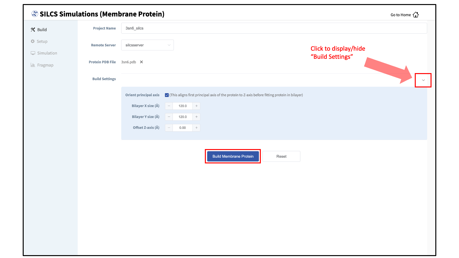
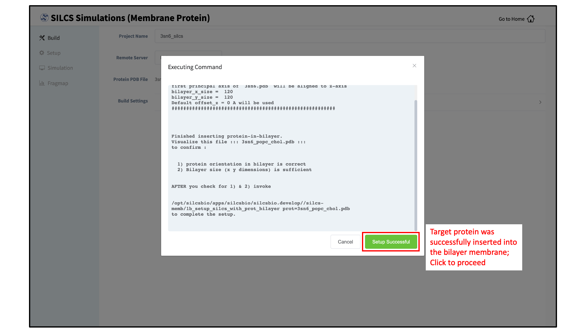
Once all information is entered correctly, press the “Build Membrane Protein” button at the bottom of the page. This will execute the utility to build the protein/bilayer system, with the bilayer consisting of 9:1 POPC:chelesterol. By default, this utility will align the first principal axis of the protein with the bilayer normal (Z-axis) and translate the protein center of mass to the center of the bilayer (Z=0). Additionally, the default system size is set to 120 Å along the X and Y dimensions. These settings can be changed under “Build Settings”.
After the protein is inserted into the bilayer, the resulting protein/bilayer system will be output in a PDB file with suffix
_popc_chol, and the page will update. Click on the green “Setup Successful” button to return to the GUI.Tip
Build Settings options during setup allow you to change the alignment of the first principal axis of the protein to the Z-axis before fitting the protein to the bilayer (default: on), the bilayer size in the X dimension (default 120 Å), the bilayer size in the Y dimension (default 120 Å), and the offset of the relative position of the protein with respect to the position of the bilayer (default 0 Å). The offset of the protein may be selected in accordance with a recommendation from an external program such as the OPM server. Please see How do I fit my membrane protein in a bilayer as suggested by the OPM server? for additional information.
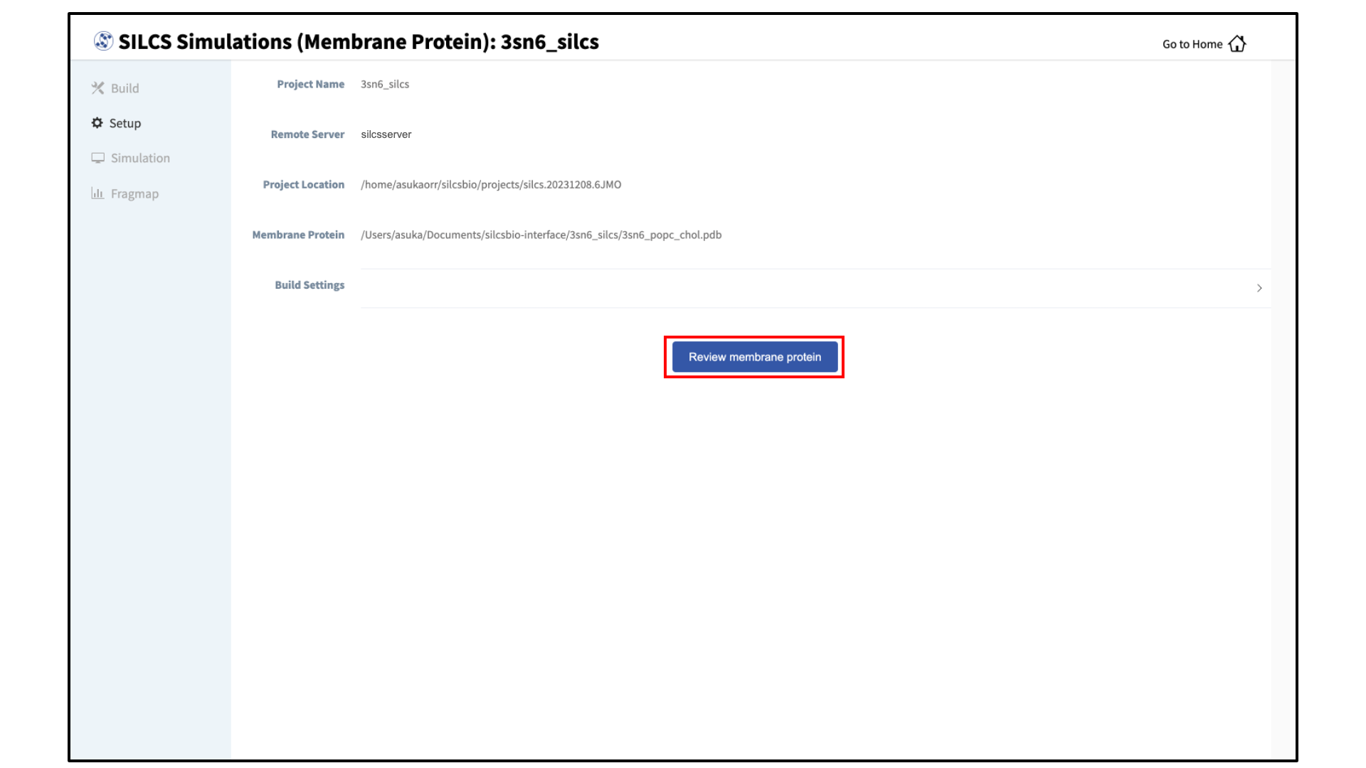
Review the built membrane protein:
After the protein is inserted into the bilayer, the GUI will prompt you to review the membrane protein. Click the “Review membrane protein” button to proceed.
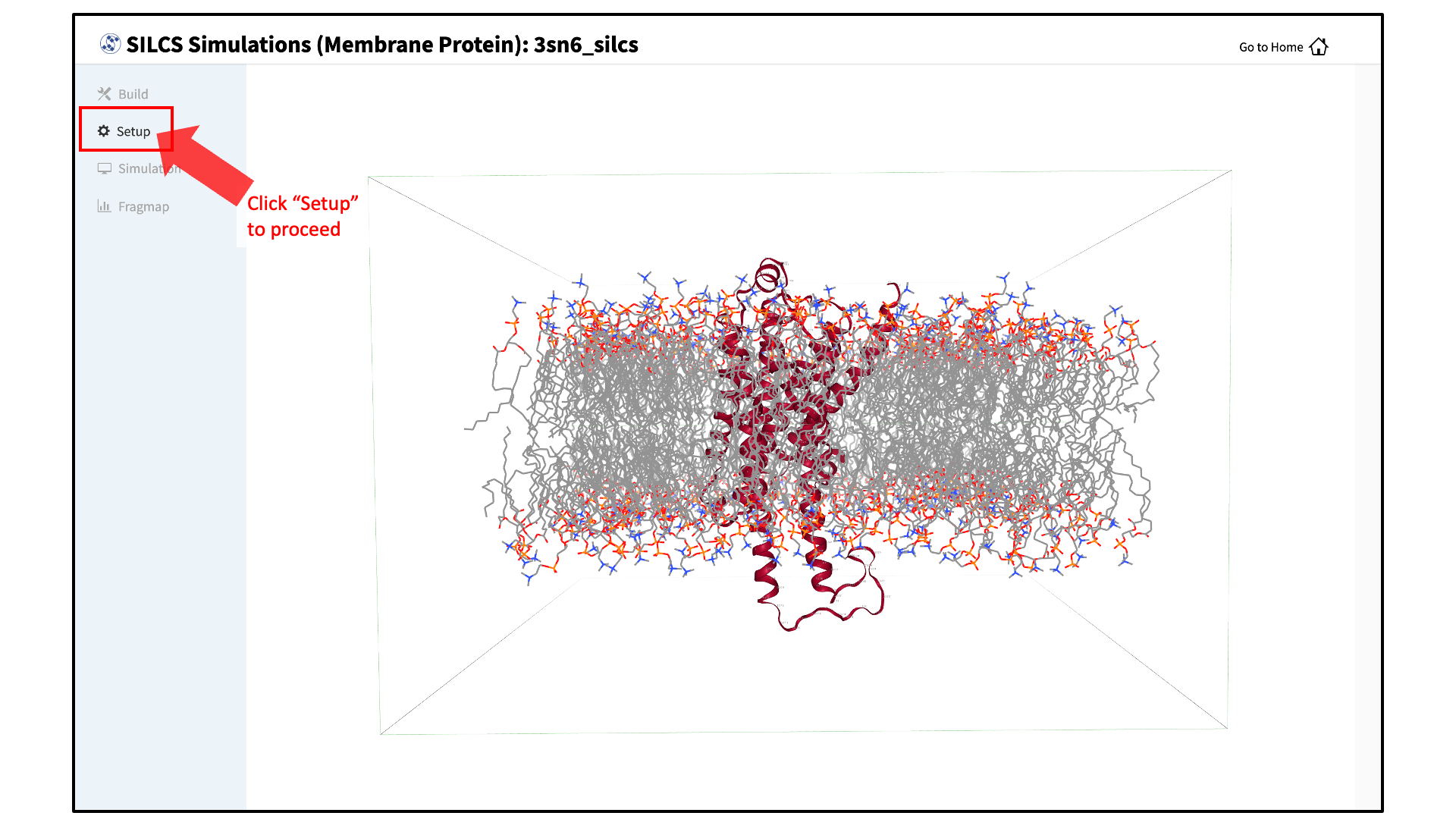
The GUI will then show you the modeled protein/bilayer system through a visualization window. Please confirm that the protein/bilayer system is correct. After reviewing the membrane protein, click “Setup” to proceed
Set up the SILCS simulations:
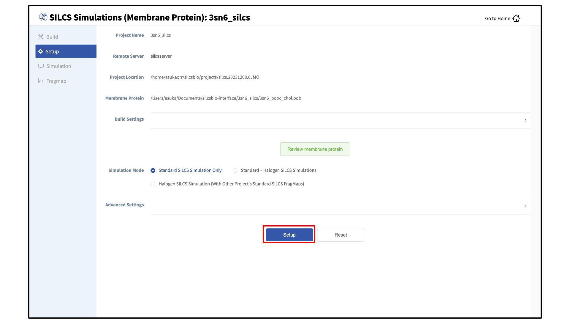
After reviewing the protein/bilayer system, the GUI will allow you to finalize setting up the SILCS simulations. During this step, you will need to decide whether to run a Standard SILCS Simulation, Standard + Halogen SILCS Simulations, or a Halogen SILCS Simulation (with another project’s Standard SILCS FragMaps). All functionality in the SILCS platform requires FragMaps from a Standard SILCS Simulation. FragMaps from Halogen SILCS Simulations can supplement Standard SILCS FragMaps for SILCS-MC: Ligand Optimization and for SILCS-MC: Docking and Pose Refinement. Visualization of Halogen SILCS FragMaps can be very useful for qualitatively informing ligand design (see Visualizing SILCS FragMaps). See FragMap names and underlying probe atoms for a complete listing of both Standard and Halogens SILCS probe molecules and the resulting FragMaps.
Note
Running a Halogen SILCS simulation requires the same computation time as running a Standard SILCS simulation, so selecting “Standard + Halogen SILCS Simulations” will consume double the computational resources as selecting “Standard SILCS Simulation”. The default is to generate and run 10 systems each for a Standard SILCS simulation and for a Halogen SILCS simulation. Therefore, if your computing resource has 10 nodes, it will take twice as much wall time to complete a “Standard + Halogen SILCS Simulations” job as to complete a “Standard SILCS Simulation”. However, if you have access to 20 nodes simultaneously, the wall time will be the same, since each individual system is run independently of the others.
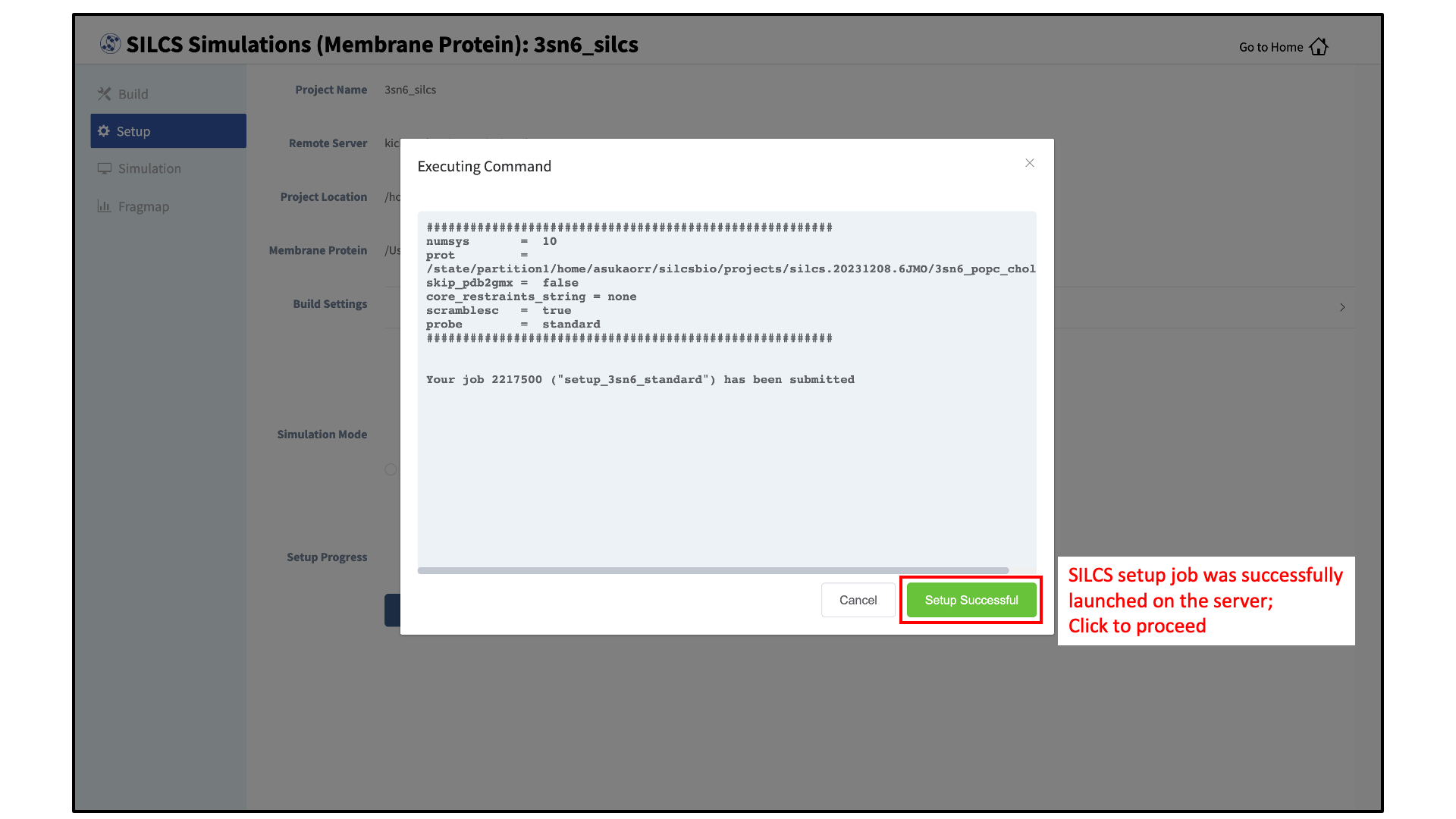
To proceed to preparing the simulation box, click “Setup”. This will submit a job on the server to prepare the SILCS simulation box by adding water and probe molecules to the protein/bilayer system. The GUI will indicate if the job was successfully launched on the server with a “Setup Successful” button. Click the “Setup Successful” button to proceed.
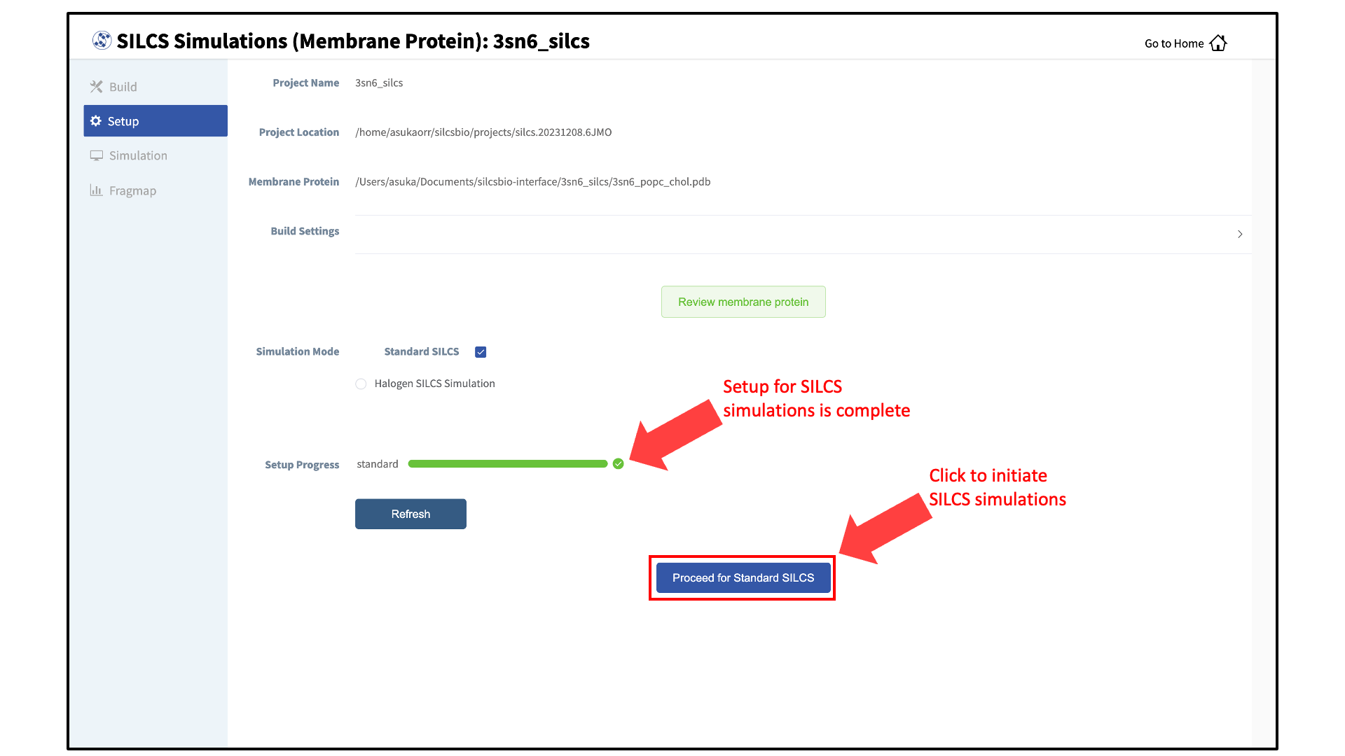
The SILCS simulation setup progress from the server will be displayed on the GUI. Once the SILCS simulation box is successfully set up, and the job is complete, a green checkmark will appear next to the progress bar. Upon completion of the SILCS simulation setup, click the “Proceed for Standard SILCS” button to continue.
Launch SILCS simulations:
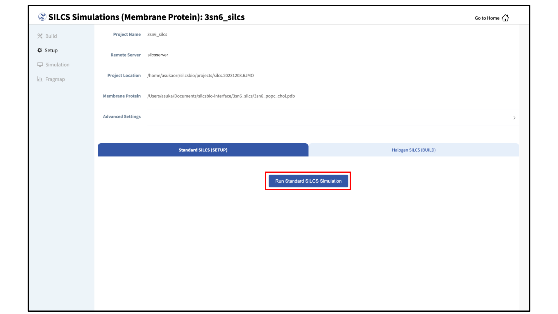
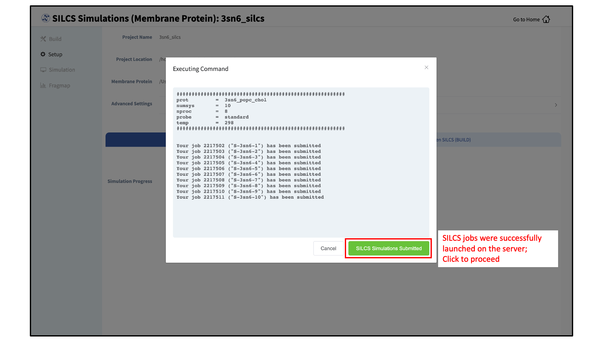
The SILCS GCMC/MD simulations can now be launched by clicking the “Run Standard SILCS Simulation” button. The SILCS GCMC/MD will begin with a 6-step pre-equilibration to slowly relax the bilayer followed by 10 ns of relaxation of the protein into the bilayer prior to the production simulation. The GUI will indicate when the SILCS jobs are successfully launched on the server with a green “SILCS Simulations Submitted” button. At this point, the jobs will continue running on the server, and it is safe to exit the GUI.
Tip
Membrane protein simulation systems are typically large and may require significant storage space (> 200 GB) and simulation time (>14 days with GPU).
FragMap generation from the GCMC/MD simulations data follows the same protocol as for non-bilayer systems (i.e., for globular proteins). Refer to previous instructions as described in SILCS Simulations Using the GUI.
If you encounter a problem, please contact support@silcsbio.com.
SILCS-Membrane Simulations Using the CLI
Prepare the input protein/bilayer system:
You may use either a bare protein structure or your own pre-built protein/bilayer system with SILCS.
If you are beginning with a bare protein, SilcsBio provides a command line utility to embed transmembrane proteins, such as GPCRs, in a bilayer of 9:1 POPC/cholesterol for subsequent SILCS simulations:
${SILCSBIODIR}/silcs-memb/1a_fit_protein_in_bilayer prot=<Protein PDB>This command will align the first principal axis of the protein with the bilayer normal (Z-axis) and translate the protein center of mass to the center of the bilayer (Z=0). The full list of parameters can be reviewed by running the command without any arguments.
Required parameter:
Path and name of the input PDB file:
prot=<protein PDB file>
Optional parameters:
Apply principal axis-based alignment:
orient_principal_axis=<true/false; default=true>
When set to true, first principal axis of the protein is aligned to Z-axis before fitting the protein in bilayer. If the protein is already oriented as desired,
orient_principal_axis=falsewill suppress the automatic principal axis-based alignment.Simulation system size:
bilayer_x_size=<default=120>
bilayer_y_size=<default=120>
By default the system size is set to 120 Å along the X and Y dimensions. To change the system size, use the
bilayer_x_sizeandbilayer_y_sizeparameters.Position of protein with respect to the bilayer:
offset_z=<Protein Z-offset distance; default=0>
By default, SILCS fits the bare protein into the lipid bilayer such that the center of mass of the protein is aligned with the center of mass of the bilayer. This may not be the best choice for your membrane proteins, and you may therefore want to adjust the position of your protein according to a recommendation from an external program such as the OPM server. In this case you can adjust the relative position of the protein with respect to the position of the bilayer by using the
offset_zoption to specify the distance by which the center of mass of the protein should be offset in Z-direction from the center of the bilayer.Note
For example, to use OPM server (https://opm.phar.umich.edu/ppm_server) output as your guide to build a transmembrane system for SILCS simulation, please see How do I fit my membrane protein in a bilayer as suggested by the OPM server?
Distance cutoff defining steric clashes:
cutoff=<cutoff for bilayer to be deleted within cutoff distance of protein; default=3.0>
To avoid unfavorable steric clashes between the protein and the modeled bilayer, bilayer molecules within the distance defined by the
cutoffparameter of the protein atoms will be deleted.
The resulting protein/bilayer system will be output in a PDB file with suffix
_popc_chol. It is important to use molecular visualization software at this stage to confirm correct orientation of the protein and size of the bilayer before using this output as the input in the next step.Alternatively, you may use a protein/bilayer system that has been built using other software tools.
Prepare the SILCS simulation box:
The following command will prepare the SILCS simulation box by adding water and probe molecules to the protein/bilayer system:
${SILCSBIODIR}/silcs-memb/1b_setup_silcs_with_prot_bilayer prot=<Protein/bilayer PDB>Tip
You may use
batch=falseoption to run this step on your head node. Note that it can sometimes take few hours to finish this step for very large systems.Required parameter:
Path and name of the input PDB file:
prot=<protein PDB file>
Optional parameters:
Number of independent simulation systems:
numsys=<# of simulations; default=10>
Skip the
pdb2gmxGROMACS utility:skip_pdb2gmx=<true/false; default=false>
Path and name of bound cofactor Mol2:
lig=<lig.mol2; default=empty/NULL>
If the input structure contains a cofactor and you wish to compute your FragMaps in the presence of the cofactor, remove the cofactor from the input PDB file and provide a separate Mol2 file of the cofactor in the correct position and orientation with respect to the target protein. Provide the path and name of the cofactor Mol2 file using the
ligparameter.Note
If your input structure contains a metal ion, please see What happens when I set up SILCS simulations with an input structure containing a metal ion?
Application of weak harmonic positional restraints:
core_restraints_string=<restrained residues, e.g., "r 17-21 | r 168-174"; default=all>
By default, a weak harmonic positional restraint, with a force constant of ~0.1 kcal/mol/Å2, is applied to all C-alpha atoms during SILCS simulations. This option lets you modify this default.
For example, if
core_restraints_string="r 17-160 | r 168-174"is supplied, then only the C-alpha atoms in residues 17 to 160 and residues 168 to 174 will be restrained.Re-orientation of residue side chains:
scramblesc=<true/false; default=true>
When set
scramblesc=true, the side chain dihedrals of the protein residues will be re-oriented.SILCS probes with halogen-containing functional groups:
halogen=<true/false; default=false>
SILCS simulations can be performed with SILCS probes that contain halogen-containing functional groups by including
halogen=true. See Setup with halogen probes for more details.Submit job to queuing system:
batch=<true/false; default=true>
This step is submitted to the queuing system by default. To run this step on the head node, use
batch=false.
Run SILCS-Membrane GCMC/MD simulations:
SILCS GCMC/MD simulations can now be launched with the following command:
${SILCSBIODIR}/silcs/2a_run_gcmd prot=<Protein/bilayer PDB> memb=trueRequired parameter:
Path and name of the input protein PDB file:
prot=<protein PDB file>
Follow SILCS-simulation protocol for membrane proteins:
memb=true
The
memboption must be set totruefor SILCS simulations of membrane proteins.
Optional parameters:
Simulation temperature:
temp=<simulation temperature; default=298>
The input simulation temperature should be entered in Kelvin units. By default, the temperature is set to 298 K.
Number of cores per simulation:
nproc=<# of cores per simulation; default=8>
Generate input files without submitting jobs to the queue:
batch<only generate inputs and not submit jobs true/false; default=false>
Use halogen probes:
halogen=<use halogen probes; true/false; default=false>
The SILCS simulation will be performed with halogen probes when
halogen=true. For more information, please refer to Setup with halogen probes.
The SILCS GCMC/MD will begin with a 6-step pre-equilibration to slowly relax the bilayer followed by 10 ns of relaxation of the protein into the bilayer prior to the production simulation.
Tip
Membrane protein simulation systems are typically large and can require significant storage space (> 200 GB) and simulation time (> 14 days with GPUs).
Generate FragMaps:
FragMap generation from the GCMC/MD simulations data follows the same protocol as for non-bilayer systems. Refer to previous instructions for
$SILCSBIODIR/silcs/2b_gen_mapsand$SILCSBIODIR/silcs/2c_fragmap.
If you encounter a problem, please contact support@silcsbio.com.
For RNA
Background
SILCS-RNA has been developed to tailor the SILCS methodology towards targeting RNA molecules with small molecules. The fundamental idea of complementarity between the functional groups in a small molecule and the binding site of the target, originally developed for protein targets, has been further developed and validated for RNA targets. Extensions to the method include an enhanced oscillating excess chemical potential protocol for the Grand Canonical Monte Carlo calculations and individual simulations of the neutral and charged solutes from which the SILCS functional group affinity maps (FragMaps) are calculated for subsequent binding site identification, pharmacophore, docking etc. calculations. Development and validation of SILCS-RNA has taken into consideration the complexities of RNA tertiary structure and the effects of the highly negatively charged phosphate backbone on sampling of neutral and charged probes. Full details have been published in [14].
SILCS-RNA Simulations Using the SilcsBio GUI
The steps for running SILCS-RNA with SilcsBio GUI are:
Begin a new SILCS-RNA project:
To begin a new SILCS-RNA project, select New SILCS project from the Home page as described in SILCS Simulations Using the GUI and select “RNA”.
Enter a project name, select the remote server, and upload input files:
Enter a project name and select the remote server where the SILCS-RNA simulation jobs will run. Additionally, provide the RNA input file. You may choose the RNA input file from the computer where you are running the SilcsBio GUI (“localhost”) or from any server you have previously configured, as described in File and Directory Selection.
If the GUI detects missing non-hydrogen atoms, non-standard residue names, or non-contiguous residue numbering, it will inform the user and provide a button labeled “Fix?”. If this button is clicked a new PDB file with these problems fixed and with the suffix
_fixedadded to the base name will be created and used. The SilcsBio GUI will not model residues that are completely missing from the PDB or loops.Warning
SILCS-RNA requires a clean input RNA PDB file for the best results. The input RNA PDB file should meet the following criteria:
The input file should NOT include ion, solvent, or water molecules
The input file should only contain one MODEL. For example, PDB files from NMR studies may contain multiple models. In this case, the user must remove unwanted models and keep only one.
The input file should NOT contain any alternate conformations of residues.
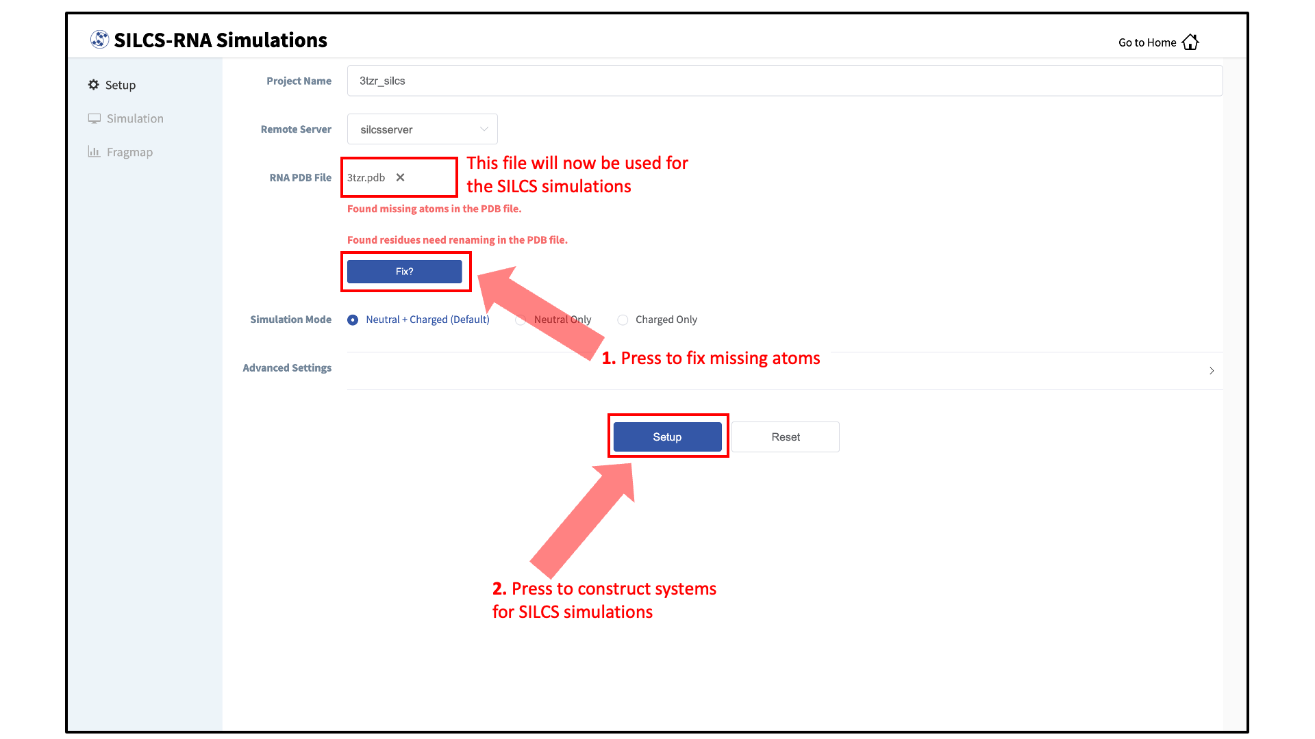
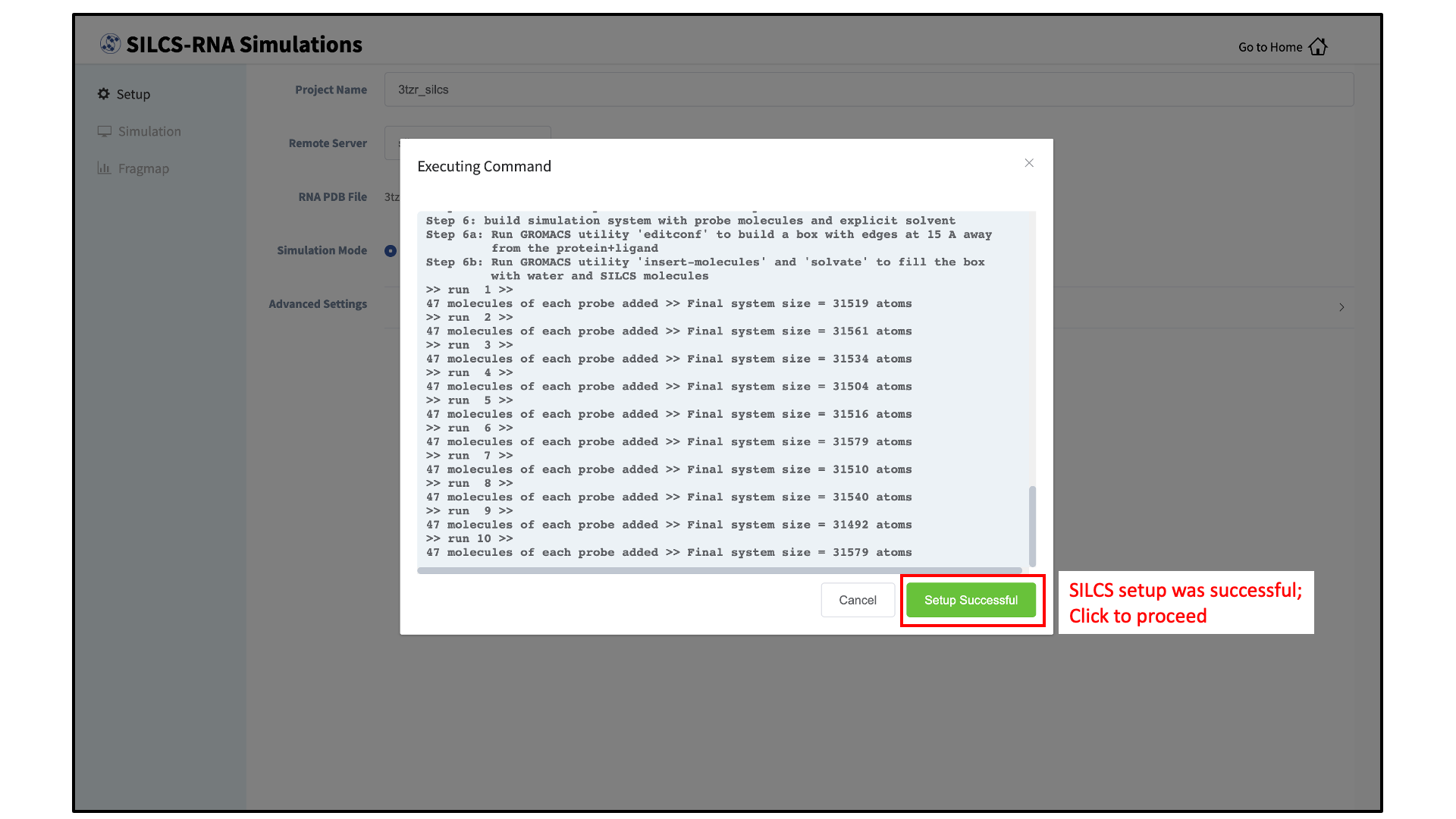
Set up SILCS simulations:
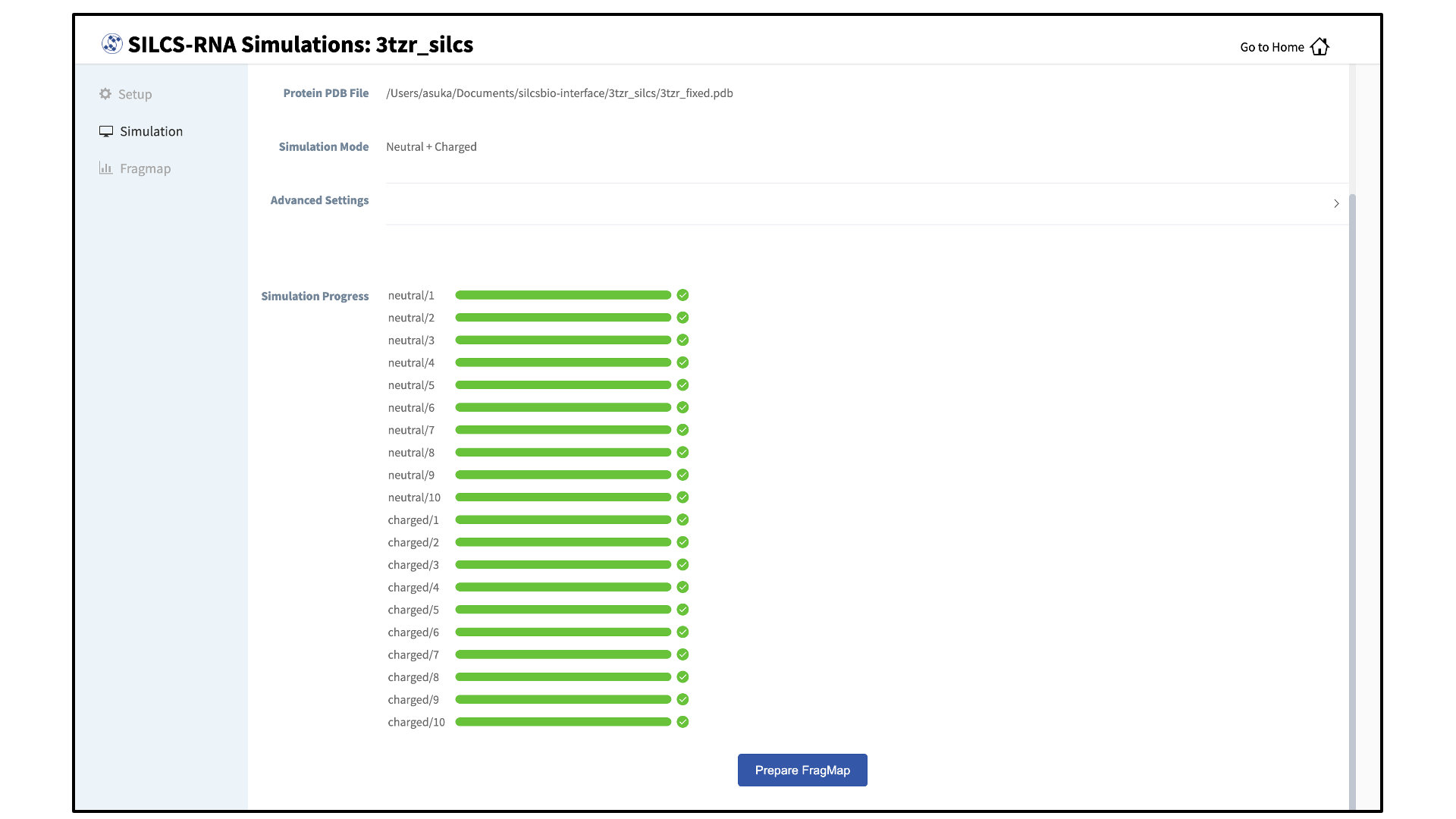
Click the “Setup” button at the bottom of the page. The GUI will contact the remote server and perform the SILCS GCMC/MD setup process. During setup, the program automatically performs several steps: The topology of the simulation system is built and probe molecules are inserted around the RNA target. This process will produce 20 PDB files required as initial structures for the simulations and can take up to 10 minutes depending of the system size. In contrast to standard SILCS with protein targets, SILCS-RNA simulations split the GCMC/MD simulations into two separate sets, one having neutral probes and the other having charged probes. A green “Setup Successful” button will appear once the process has been successfully completed. Click the green “Setup Successful” button to proceed.
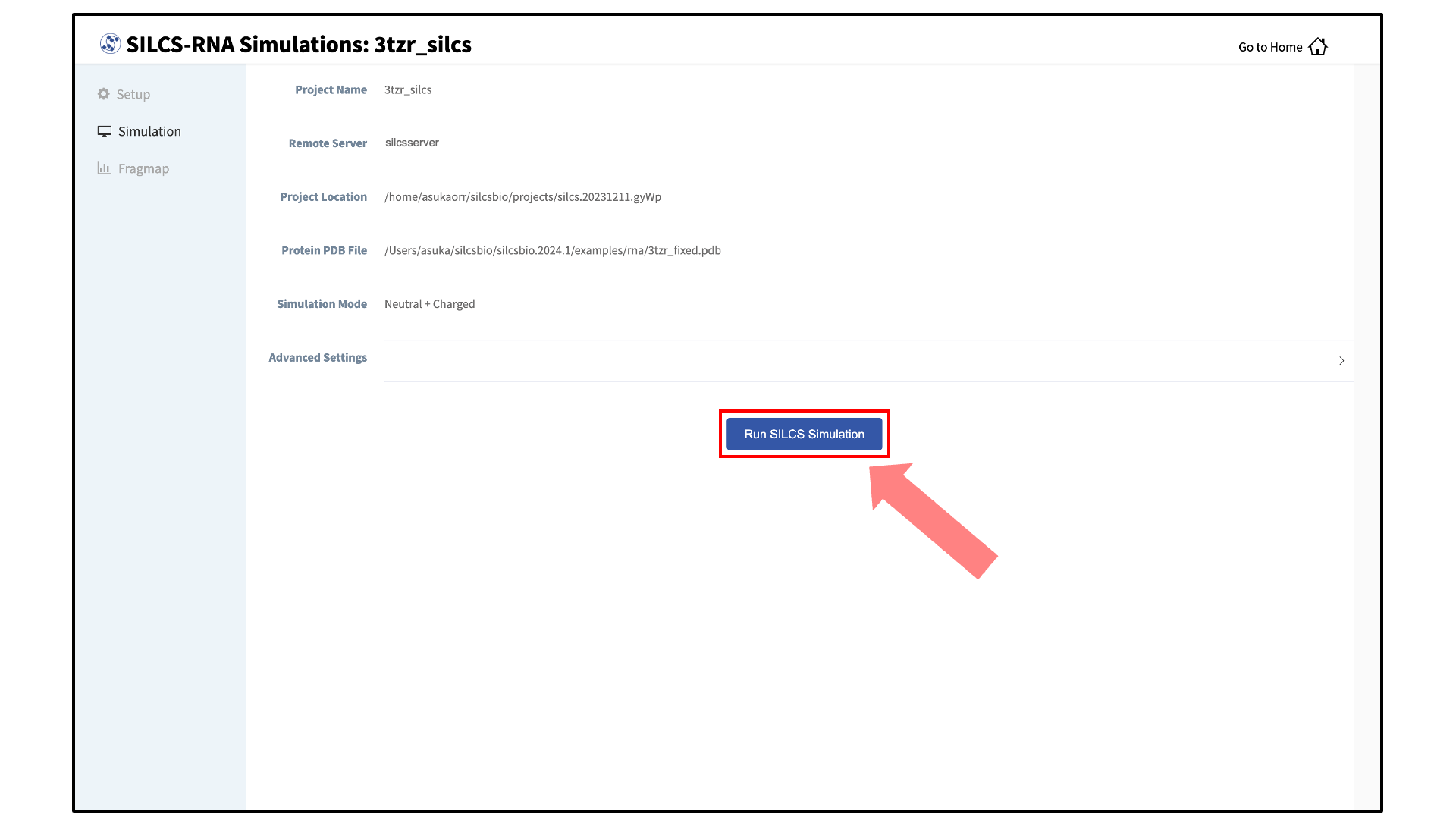
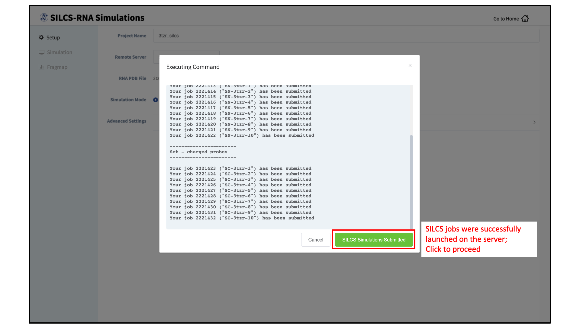
Launch SILCS simulations:
Your SILCS-RNA GCMC/MD simulations can now be started by clicking the “Run SILCS Simulation” button. This will submit 20 compute jobs to the queueing system on the server. The GUI will indicate when the SILCS jobs are successfully launched on the server with a green “SILCS Simulations Submitted” button. At this point, the jobs will continue running on the server, and it is safe to exit the GUI.
Tip
Before running your SILCS simulations, you may wish to double check that you have selected the desired file folder on the remote server and that it has 100+ GB of storage space available.
Generate FragMaps:
Once your SILCS-RNA simulations are finished, the GUI can be used to create FragMaps and visualize them. Green progress bars indicate that the simulations have been successfully completed. Once all progress bars are green, the “Prepare FragMap” button will appear.
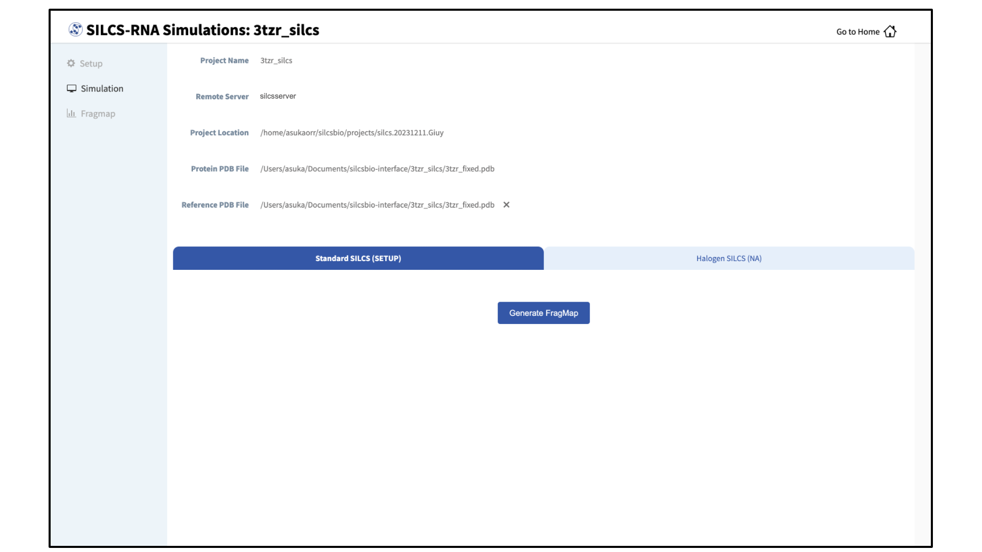
Press the “Prepare FragMap” button, and on the next screen, confirm your “Reference PDB File”. FragMaps will be created in the coordinate reference frame of this file. Generally, this reference PDB file is the same as the initial input PDB file. A different PDB file of the same RNA structure may be used to generate FragMaps relative to that orientation. Click “Generate FragMap” to generate FragMaps and download them to the local computer for visualization.
Note
SILCS-RNA currently does not support Halogen SILCS simulations.
Processing the GCMC-MD trajectories will take 10-20 minutes, with the GUI providing updates on progress from the server during this process. Once completed, the GUI will automatically copy the files from the server onto the local computer and load them for visualization. Please see Visualizing SILCS FragMaps for details on how to use the SilcsBio GUI, as well as external software (MOE, PyMol, VMD), to visualize SILCS FragMaps.
As with FragMaps for protein targets, your SILCS-RNA FragMaps for RNA targets can be used for detecting hotspots and performing fragment-based drug design (SILCS-Hotspots), creating pharmacophore models (SILCS-Pharm), docking ligands and refining existing docked poses (SILCS-MC: Docking and Pose Refinement), and optimizing lead compounds (SILCS-MC: Ligand Optimization).
SILCS-RNA Simulations Using the CLI
Prepare the input RNA PDB file:
SILCS-RNA requires a clean input RNA PDB file for best results. The input RNA PDB file should meet the following criteria:
The input file should NOT include ion, solvent, or water molecules
The input file should only contain one MODEL. For example, PDB files from NMR studies may contain multiple models. In this case, the user must remove unwanted models and keep only one.
The input file should NOT contain any alternate conformations of residues.
Set up the SILCS-RNA simulations:
${SILCSBIODIR}/silcs-rna/1_setup_silcs_boxes prot=<RNA PDB file>To determine if the setup is complete, check that the 20 PDB files required for the simulations are available using the command
ls 1_setup_*/*_silcs.*.pdbIt is also a good idea to visualize these files to confirm the presence of the RNA molecule and the SILCS solute molecules (probes) within a box of water molecules. In contrast to standard SILCS with protein targets, SILCS-RNA simulations split the GCMC/MD simulations into two separate sets, one having neutral probes (1_setup_neutral) and the other having charged probes (1_setup_charged).The setup command offers a number of options. The full list of parameters can be reviewed by running the command without any arguments.
Required parameter:
Path and name of the input RNA PDB file:
prot=<RNA PDB file>
Optional parameters:
Number of independent simulation systems per set of probes:
numsys=<# of simulations; default=10>
SILCS simulations, by default, consist of 10 replicate simulations per set of probes, each with different initial velocities, to enhance sampling. SILCS-RNA simulations consist of two sets of probes, one set of uncharged probes and one set of charged probes. Thus, with both sets of probes having 10 replicate simulations, by default, 20 simulation systems will be set up (2 set of probes * 10 simulations = 20 simulations). The number of simulations can be adjusted using the
numsyskeyword, and the resulting number of simulations will be 2 *numsys.Skip the
pdb2gmxGROMACS utility:skip_pdb2gmx=<true/false; default=false>
Sets of probe molecules:
sets=<neutral+charged/neutral/charged; default="neutral+charged">
Due to the highly negatively charged phosphate backbone of RNAs, SILCS-RNA uses two sets of probe molecules (one set of charged probes and one set of neutral probes) by default. The use of only one set of probe molecules may be specified with the
setskeyword.Path and name of bound ligand Mol2:
lig=<lig.mol2; default=empty/NULL>
If the input structure contains a bound ligand and you wish to compute your FragMaps in the presence of the ligand, remove the ligand from the input PDB file and provide a separate Mol2 file of the ligand in the correct position and orientation with respect to the target protein. Provide the path and name of the ligand Mol2 file using the
ligkeyword.Simulation box size:
margin=<system margin (Å); default=15>
By default, the simulation system size is determined by adding a 15 Å margin to the size of the input protein structure. The size of the simulation box can be customized by using the
marginkeyword.
Note
As in standard SILCS simulations, a weak harmonic positional restraint, with a force constant of ~0.1 kcal/mol/Å2, is applied to all MG, C1’, URA-N3, CYT-N3, ADE-N1 and GUA-N1 atoms during simulations. The option to change this default is not available in the current version of SILCS-RNA.
Warning
The setup program internally uses the GROMACS utility
pdb2gmx, which may have problems processing the RNA PDB file. The most common reasons for errors at this stage involve mismatches between the expected residue name/atom names in the input PDB and those defined in the CHARMM force-field.To fix this problem: Run the
pdb2gmxcommand manually from within the1_setup_neutralAND the1_setup_chargeddirectories for detailed error messages. For guidance on syntax, the setup script already prints out the exact commands you need to run:cd 1_setup_neutral pdb2gmx –f <RNA PDB NAME>_4pdb2gmx.pdb –ff charmm36 –water tip3p –o test.pdb –p test.top -ter -merge all cd ../1_setup_charged pdb2gmx –f <RNA PDB NAME>_4pdb2gmx.pdb –ff charmm36 –water tip3p –o test.pdb –p test.top -ter -merge all cd ..
Once all errors in the input PDB are corrected, rerun the setup script with
skip_pdb2gmx=true.Note
SILCS-RNA currently does not support Halogen SILCS simulations.
Submit the SILCS-RNA GCMC/MD simulations:
Following completion of the setup, start the 20 GCMC/MD jobs:
${SILCSBIODIR}/silcs-rna/2a_run_gcmd prot=<RNA PDB file>Required parameter:
Path and name of the input RNA PDB file:
prot=<RNA PDB file>
Optional parameters:
Simulation temperature:
temp=<simulation temperature; default=298>
The input simulation temperature should be entered in Kelvin units. By default, the temperature is set to 298 K.
Number of cores per simulation:
nproc=<# of cores per simulation; default=8>
Generate input files without submitting jobs to the queue:
batch<only generate inputs and not submit jobs true/false; default=false>
This script will submit 20 jobs to the predefined queue. Each job runs 100 ns of GCMC/MD with the RNA and the solute molecules; 10 jobs are with neutral solute molecules (probes), and 10 are with charges solute molecules (probes).
Tip
SILCS simulations are run at a temperature of 298 K by default. It is possible to set a custom temperature by adding the
temp=<simulation temperature; default=298>option to the2a_run_gcmdcommand. For example,temp=310would run the SILCS simulations at 310 K.Once the simulations are complete, the
2a_run_gcmd_neutral/[1-10]AND2a_run_gcmd_charged/[1-10]directories will contain*.prod.100.rec.xtctrajectory files. If these files are not generated, then your simulations are either still running or stopped due to a problem. Look in the log files within these directories to diagnose problems.To check job progress, use the following command:
${SILCSBIODIR}/silcs-rna/check_progressThis will provide a summary list of the SILCS jobs consisting of the job path, the job number, the task ID, the job status, and the current/total number of GCMC/MD cycles. Job status values are: Q [queued], R [running], E [successfully ended], F [failed], NA [not submitted].
Generate FragMaps:
Once your simulations are done, generate the SILCS FragMaps using the following command:
${SILCSBIODIR}/silcs-rna/2b_gen_maps prot=<RNA PDB file>Required parameter:
Path and name of the input RNA PDB file:
prot=<RNA PDB file>
Optional parameters:
Simulation box size:
margin=<size of margin in the map; default=10>
Reference structure:
ref=<reference PDB; default=same PDB file given in prot>
By default, the FragMaps will be oriented around the protein structure that was used as the initial structure for the SILCS simulations. The FragMaps can also be oriented around a different structure by specifying it with
ref=.Spacing between voxels:
spacing=<map spacing; default=1.0>
The probabiliy of each functional group occupying a voxel is used to calculate GFE values. By default, the spacing between each voxel is 1.0 Å.
First cycle number to use for map generation:
begin=<cycle number to begin for map generation; default=1>
Last cycle number to use for map generation:
end=<cycle number to end for map generation; default=100>
This script will submit 20 jobs to the predefined queue. Each job runs 100 ns of GCMC/MD with the RNA and the solute molecules; 10 jobs are with neutral solute molecules (probes), and 10 are with charges solute molecules (probes).
This will submit 20 single-core jobs that will build occupancy maps (FragMaps) spanning the simulation box for select solute molecule atoms representing different functional groups. For a ~50K atom simulation system, this step takes approximately 10-20 minutes to complete. The FragMaps have a default grid spacing of 1 Å.
The next step is to combine the occupancy FragMaps generated from individual simulations and convert them into GFE FragMaps. Each voxel in a GFE FragMap contains a Grid Free Energy (GFE) value for the probe type that was used to create the corresponding occupancy FragMap.
${SILCSBIODIR}/silcs-rna/2c_fragmap prot=<RNA PDB file>Required parameter:
Path and name of the input RNA PDB file:
prot=<RNA PDB file>
Optional parameters:
Simulation temperature:
temp=<simulation temperature; default=298>
If the simulation temperature was specified for
2a_run_gcmd, please specify the same temperature for this step using thetempparameter. The input simulation temperature should be entered in Kelvin units. By default, the temperature is set to 298 K.Skip overlap coefficient calculation:
skipoc=<true/false; skip overlap coefficient calculation; default=false>
Generate maps in CNS format:
cns=<true/false; generate maps in CNS format; default=false>
First cycle number to use for map generation:
begin=<cycle number to begin for map generation; default=1>
Last cycle number to use for map generation:
end=<cycle number to end for map generation; default=100>
GFE FragMaps will be created in the
silcs_fragmap_<RNA PDB NAME>/mapsdirectory, and PyMOL and VMD scripts to load these file will be created in thesilcs_fragmap_<RNA PDB NAME>directory. Please see Visualizing SILCS FragMaps for details on how to use the SilcsBio GUI, as well as external software (MOE, PyMol, VMD), to visualize SILCS FragMaps.As with FragMaps for protein targets, your SILCS-RNA FragMaps for RNA targets can be used for detecting hotspots and performing fragment-based drug design (SILCS-Hotspots), creating pharmacophore models (SILCS-Pharm), docking ligands and refining existing docked poses (SILCS-MC: Docking and Pose Refinement), and optimizing lead compounds (SILCS-MC: Ligand Optimization).
Cleanup:
Raw trajectory output files are large. To reduce disk usage due to these files, use the cleanup command:
${SILCSBIODIR}/silcs-rna/2d_cleanup prot=<RNA PDB file>Required parameter:
Path and name of input RNA PDB file:
prot=<RNA PDB file>
Optional parameters:
Number of simulation systems:
numsys=<# of simulations; default=10>
Delete original files:
delete=<delete original files after tar-balls are created true/false; default=false>
The
2d_cleanupcommand deletes unnecessary files, such as those from the equilibration phase, and deletes hydrogen atoms from production trajectory files for each run directory,1/,2/, etc. It then creates a.tar.gzfile of that directory. That is to say, the contents of1.tar.gzand1/after running cleanup are identical. You may choose to remove either one of those without loss of information, though we strongly recommend comparing the output oftar tvzf <run>.tar.gzwith the output offind <run> -type f, where you replace<run>with1,2, etc. and confirm the contents are identical before deleting anything.